Krylovova kvantová diagonalizace mřížkových Hamiltonů

Odhadovaný čas: 70 minut na procesoru Heron nebo Nighthawk (POZNÁMKA: Jedná se pouze o odhad. Skutečný čas se může lišit.)

Výsledky učení

• Jak interpretovat Krylovovu kvantovou diagonalizaci (KQD) jako učení konečné Hamiltonovské funkce, která funguje jako spektrální filtr.

• Jak sestavit projektovaný Hamiltonián a matice překryvu pomocí rozšířených swap-test měření.

• Jak vyřešit výsledný zobecněný problém vlastních čísel (GEVP) a získat odhad energie základního stavu pro mřížkový Hamiltonián.

Předpoklady

• Qiskit primitiva

• Odhad energie základního stavu Heisenbergova řetězce pomocí VQE

• Kurz algoritmů kvantové diagonalizace

Pozadí

Tento tutoriál ukazuje, jak implementovat algoritmus Krylovovy kvantové diagonalizace (KQD) v rámci vzorů Qiskitu. Nejprve se dozvíš teorii za algoritmem a pak uvidíš ukázku jeho spuštění na QPU.

Odhad nízkoenergetických vlastností mnohatělesových Hamiltoniánů je klíčovým úkolem v kvantové simulaci. Například energie základního stavu a nízko položené excitace přímo souvisí s chemickou stabilitou, magnetickým uspořádáním, kvantovými fázovými přechody a odezvou materiálu. Na klasickém počítači roste dimenze Hilbertova prostoru exponenciálně s počtem orbitalů nebo spinů, takže přímá diagonalizace se rychle stává nepraktickou.

Existuje několik přístupů kvantového počítání k tomuto problému. Blízkodobé variační metody, jako je variační kvantový eigensolver (VQE), používají relativně mělké parametrizované obvody, ale vyžadují nelineární klasickou optimalizační smyčku s mnoha vyhodnoceními kvantového obvodu. Na druhé straně odhad kvantové fáze (QPE) poskytuje přímější cestu k odhadu vlastních čísel s rigorózními zárukami, ale standardní QPE vyžaduje dlouhé koherentní obvody a je vhodný především pro odolné kvantové počítače. KQD stojí mezi těmito dvěma přístupy: používá vývoj Hamiltoniánu v reálném čase, jako u algoritmů založených na odhadu fáze, ale nahrazuje úplný odhad fáze kompaktním projektovaným problémem vlastních čísel, který lze řešit klasicky.

Uvažujme $n$-qubitový Hamiltonián $H$ a referenční stav $\lvert \psi_{0}\rangle$. Metoda KQD sestavuje Krylovův podprostor ze stavů vyvinutých v reálném čase,

$$\begin{equation*} \lvert \psi_\ell\rangle = e^{-i\ell\Delta t H}\lvert \psi_{0}\rangle, \qquad \ell = 0,1,\ldots,r-1, \end{equation*}$$

kde $r$ je Krylovova dimenze a $\Delta t$ je časový krok. Jakýkoli stav v Krylovově podprostoru je pak reprezentován jako lineární kombinace těchto bázových stavů,

$$\begin{equation*} \lvert \psi(\mathbf{c})\rangle = \frac{\sum_{\ell=0}^{r-1} c_\ell \lvert \psi_\ell\rangle} {\left\|\sum_{\ell=0}^{r-1} c_\ell \lvert \psi_\ell\rangle\right\|}, \end{equation*}$$

where the denominator normalizes the state.

Pomocí jednoduché algebry vidíme, že odpovídající energie je zapsána jako Rayleighův podíl,

$$\begin{equation*} E(\mathbf{c}) =\langle \psi(\mathbf{c})|H|\psi(\mathbf{c}) \rangle= \frac{ \sum_{k,\ell} c_k^* c_\ell \langle \psi_k\vert H\vert\psi_\ell\rangle }{ \sum_{k,\ell} c_k^* c_\ell \langle \psi_k\vert\psi_\ell\rangle } = \frac{ \mathbf{c}^{\dagger}\mathcal{H}\mathbf{c} }{ \mathbf{c}^{\dagger}\mathcal{S}\mathbf{c} }. \end{equation*}$$

Zde matice $\mathcal{S}$ a $\mathcal{H}$,

$$\begin{equation*} \mathcal{S}_{k\ell}=\langle \psi_k\vert\psi_\ell\rangle, \qquad \mathcal{H}_{k\ell}=\langle \psi_k\vert H\vert\psi_\ell\rangle \end{equation*}$$

definují projektované matice překryvu a Hamiltoniánu. Jejich prvky se odhadují pomocí měření kvantového obvodu.

Naším cílem je najít koeficient $\mathbf{c}$, který dává minimum $E(\mathbf{c})$:

$$\begin{equation*} \min_{\mathbf{c}\neq \mathbf{0}} E(\mathbf{c}). \end{equation*}$$

Podle Rayleigh-Ritzova teorému je tato minimalizace ekvivalentní řešení zobecněného problému vlastních čísel (GEVP),

$$\begin{equation*} \mathcal{H}\mathbf{c}=E \mathcal{S}\mathbf{c}. \end{equation*}$$

Poznamenejme, že dimenze $r$ může být dostatečně malá na to, aby klasický počítač vyřešil GEVP.

Toto je stejný variační princip, jaký se používá při klasické podprostorové diagonalizaci, ale zde jsou bázové stavy generovány kvantovým časovým vývojem. Ve srovnání s VQE vyžaduje KQD obvykle hlubší obvody, protože se spoléhá na vývoj v reálném čase. Na oplátku se KQD vyhýbá nelineární optimalizaci parametrů a iterativnímu spouštění na kvantovém hardwaru a systematicky se zlepšuje s rozšiřováním projektovaného podprostoru. Tento algoritmus byl demonstrován ve velkém měřítku na existujícím kvantovém hardwaru [2] a jeho výkon lze analyzovat s prokazatelnými zárukami [1].

Požadavky

Před zahájením tohoto tutoriálu se ujisti, že máš nainstalováno následující:

• Qiskit SDK v2.3 nebo novější s podporou vizualizace

• Qiskit Runtime v0.22 nebo novější ( pip install qiskit-ibm-runtime )

• SciPy (pip install scipy)

• Matplotlib (pip install matplotlib)

• Pandas (pip install pandas)

Spuštění na hardwaru vyžaduje qiskit-ibm-runtime a přístup k účtu IBM Quantum®.

Nastavení

Buňka pro nastavení importuje potřebné moduly a definuje pomocné funkce pro workflow:

1. sestav Heisenbergův Hamiltonián;

2. vyřeš prahovaný GEVP;

3. vyhodnoť naučený Krylovův filtr;

4. převeď hodnoty filtru na spektrální váhy;

5. vykresli referenční a filtrovaná rozdělení energie.

# Added by doQumentation — required packages for this notebook
!pip install -q matplotlib numpy pandas qiskit qiskit-ibm-runtime scipy

from __future__ import annotations

import warnings

import numpy as np
import pandas as pd
import scipy.linalg as la
import matplotlib.pyplot as plt

from qiskit import QuantumCircuit, transpile
from qiskit.circuit import Parameter
from qiskit.circuit.library import PauliEvolutionGate
from qiskit.primitives import StatevectorEstimator
from qiskit.quantum_info import Operator, SparsePauliOp
from qiskit.synthesis import LieTrotter, SuzukiTrotter
from qiskit.transpiler import PassManager, Layout
from qiskit.transpiler.passes import CommutativeOptimization
from qiskit.transpiler.preset_passmanagers import generate_preset_pass_manager
from qiskit_ibm_runtime import QiskitRuntimeService, EstimatorV2, Batch
from qiskit_ibm_runtime.fake_provider import FakeMarrakesh

warnings.filterwarnings("ignore")

def make_heisenberg_hamiltonian(
    num_qubits: int,
    coupling: float = 1.0,
) -> SparsePauliOp:
    """Make a Heisenberg Hamiltonian for a 1D chain of qubits with nearest-neighbor interactions."""
    terms: list[tuple[str, complex]] = []

    def append_term(q0: int, q1: int, pauli: str):
        label = ["I"] * num_qubits
        label[num_qubits - 1 - q0] = pauli[0]
        label[num_qubits - 1 - q1] = pauli[1]
        terms.append(("".join(label), coupling))

    for pauli in ("XX", "YY", "ZZ"):
        for q in range(num_qubits - 1):
            append_term(q, q + 1, pauli)
    return SparsePauliOp.from_list(terms).simplify()

def _basis_state_transition_amplitude_sparse(
    hamiltonian: SparsePauliOp,
    bra_state: int,
    ket_state: int,
) -> complex:
    """Evaluate <bra_state|H|ket_state> for computational-basis states."""
    num_qubits = hamiltonian.num_qubits
    amplitude = 0.0 + 0.0j
    for pauli, coeff in zip(hamiltonian.paulis, hamiltonian.coeffs):
        new_state = ket_state
        phase = 1.0 + 0.0j
        for q in range(num_qubits):
            x = bool(pauli.x[q])
            z = bool(pauli.z[q])
            if not x and not z:
                continue
            bit = (new_state >> q) & 1
            if x and z:
                # Y|0> = i|1>, Y|1> = -i|0>
                phase *= 1j if bit == 0 else -1j
                new_state ^= 1 << q
            elif x:
                new_state ^= 1 << q
            else:
                # Z|0> = |0>, Z|1> = -|1>
                if bit:
                    phase *= -1
        if new_state == bra_state:
            amplitude += coeff * phase
    return amplitude

def basis_state_expectation_sparse(
    hamiltonian: SparsePauliOp,
    bitstring: str,
) -> complex:
    """Evaluate <bitstring|H|bitstring>."""
    state = int(bitstring, 2)
    return _basis_state_transition_amplitude_sparse(
        hamiltonian,
        bra_state=state,
        ket_state=state,
    )

def diagonalize_single_1_subspace(
    hamiltonian: SparsePauliOp,
) -> np.ndarray:
    """Diagonalize the Hamiltonian projected onto the single-excitation subspace."""
    num_qubits = hamiltonian.num_qubits

    # Integer basis states |...010...>, with the excitation at qubit k.
    basis = [1 << k for k in range(num_qubits)]

    h_single = np.empty((num_qubits, num_qubits), dtype=complex)

    for row, bra_state in enumerate(basis):
        for col, ket_state in enumerate(basis):
            h_single[row, col] = _basis_state_transition_amplitude_sparse(
                hamiltonian,
                bra_state=bra_state,
                ket_state=ket_state,
            )
    # Remove floating-point-level asymmetry.
    h_single = 0.5 * (h_single + h_single.conj().T)
    evals, _ = np.linalg.eigh(h_single)
    return np.real(evals)

def simple_transpilation(circuit: QuantumCircuit) -> QuantumCircuit:
    """Transpilation to simplify the circuit"""
    pm = PassManager(
        [
            CommutativeOptimization(),
        ]
    )
    circuit = transpile(circuit, optimization_level=3)
    circuit = pm.run(circuit)
    return circuit

def summarize_circuit(circuit: QuantumCircuit) -> dict[str, int | str]:
    """Summarize the circuit with depth, size, and 2-qubit gate information."""
    two_qubit_total = sum(
        inst.operation.num_qubits == 2 for inst in circuit.data
    )
    two_qubit_depth = circuit.depth(lambda x: x[0].num_qubits == 2)
    return {
        "depth": circuit.depth(),
        "size": circuit.size(),
        "2q gates": two_qubit_total,
        "2q depth": two_qubit_depth,
    }

def solve_thresholded_gevp(
    h_matrix: np.ndarray,
    s_matrix: np.ndarray,
    threshold: float = 1e-10,
) -> tuple[float, np.ndarray, int]:
    """Solve H c = E S c using canonical orthogonalization of S."""
    s_vals, s_vecs = la.eigh(s_matrix)

    valid = s_vals > threshold
    if not np.any(valid):
        raise ValueError(
            "All overlap eigenvalues were removed by thresholding."
        )

    keep = valid

    orthogonalizer = s_vecs[:, keep] @ np.diag(1.0 / np.sqrt(s_vals[keep]))
    h_orth = orthogonalizer.conj().T @ h_matrix @ orthogonalizer
    h_orth = 0.5 * (h_orth + h_orth.conj().T)

    eigvals, eigvecs = la.eigh(h_orth)

    coeffs = orthogonalizer @ eigvecs[:, 0]
    normalization = np.sqrt(np.real(coeffs.conj().T @ s_matrix @ coeffs))
    coeffs /= normalization

    return float(np.real(eigvals[0])), coeffs, int(np.sum(keep))

V první části tohoto tutoriálu demonstrujeme metodu KQD pomocí lokálního statevector simulátoru. Později použijeme reálný kvantový backend k řešení problému v užitkovém měřítku.

Také definujeme fake backend, abychom demonstrovali transpilaci specifickou pro backend a prozkoumali výsledný obvod.

try:
    service = QiskitRuntimeService()
except Exception:
    QiskitRuntimeService.save_account(
        token="<api_token>", instance="<instance>", overwrite=True
    )
    service = QiskitRuntimeService()

backend = FakeMarrakesh()

Příklad simulátoru malého měřítka

Krok 1: Mapování klasických vstupů na kvantový problém

Hamiltonián a referenční stav

Tento příklad používá 12-qubitový Heisenbergův řetězec s otevřenými hranicemi ($n=12$),

$$\begin{equation*} H=\sum_{i=0}^{n-2}\left(X_iX_{i+1}+Y_iY_{i+1}+Z_iZ_{i+1}\right), \end{equation*}$$

se stavem produktu s jedinou excitací

$$\begin{equation*} |\psi_{0}\rangle=|000001000000\rangle \end{equation*}$$

jako referenčním stavem. Protože výše definovaný Heisenbergův Hamiltonián zachovává celkový počet excitací, referenční stav zůstává v podprostoru s jedinou excitací, jehož dimenze roste pouze lineárně s počtem qubitů. Můžeme proto efektivně vypočítat přesnou energii základního stavu diagonalizací Hamiltoniánu omezeného na tento podprostor a použít ji čistě jako diagnostický benchmark pro odhad KQD. Samotný workflow KQD odhaduje projektované prvky matice pomocí Qiskit primitiv a výsledný projektovaný problém řeší klasicky.

# Problem definition for the simulator example
num_qubits = 12
hamiltonian = make_heisenberg_hamiltonian(num_qubits=num_qubits, coupling=1.0)
ref_bitstring = "000001000000"
ref_energy = basis_state_expectation_sparse(hamiltonian, ref_bitstring)

print("Hamiltonian:")
print(hamiltonian)
print(f"Reference state: |{ref_bitstring}>")
print("Reference energy: ", ref_energy)

Hamiltonian:
SparsePauliOp(['IIIIIIIIIIXX', 'IIIIIIIIIXXI', 'IIIIIIIIXXII', 'IIIIIIIXXIII', 'IIIIIIXXIIII', 'IIIIIXXIIIII', 'IIIIXXIIIIII', 'IIIXXIIIIIII', 'IIXXIIIIIIII', 'IXXIIIIIIIII', 'XXIIIIIIIIII', 'IIIIIIIIIIYY', 'IIIIIIIIIYYI', 'IIIIIIIIYYII', 'IIIIIIIYYIII', 'IIIIIIYYIIII', 'IIIIIYYIIIII', 'IIIIYYIIIIII', 'IIIYYIIIIIII', 'IIYYIIIIIIII', 'IYYIIIIIIIII', 'YYIIIIIIIIII', 'IIIIIIIIIIZZ', 'IIIIIIIIIZZI', 'IIIIIIIIZZII', 'IIIIIIIZZIII', 'IIIIIIZZIIII', 'IIIIIZZIIIII', 'IIIIZZIIIIII', 'IIIZZIIIIIII', 'IIZZIIIIIIII', 'IZZIIIIIIIII', 'ZZIIIIIIIIII'],
              coeffs=[1.+0.j, 1.+0.j, 1.+0.j, 1.+0.j, 1.+0.j, 1.+0.j, 1.+0.j, 1.+0.j, 1.+0.j,
 1.+0.j, 1.+0.j, 1.+0.j, 1.+0.j, 1.+0.j, 1.+0.j, 1.+0.j, 1.+0.j, 1.+0.j,
 1.+0.j, 1.+0.j, 1.+0.j, 1.+0.j, 1.+0.j, 1.+0.j, 1.+0.j, 1.+0.j, 1.+0.j,
 1.+0.j, 1.+0.j, 1.+0.j, 1.+0.j, 1.+0.j, 1.+0.j])
Reference state: |000001000000>
Reference energy:  (7+0j)

Nastavení parametrů algoritmu

Na základě horních mezí normy Hamiltoniánu ref. [1] heuristicky navrhuje časový krok $\Delta t$ jako $\pi/\|H\|$. Protože spektrální normu $\|H\|$ je obtížné vypočítat, místo toho použijeme její horní mez:

$$\begin{equation*} \|H\| \le \sum_{i=0}^{n-2}\underbrace{\|X_i X_{i+1}+Y_{i} Y_{i+1}+Z_{i} Z_{i+1}\|}_{4 \times 4 \text{ matrix, easy to calculate the norm}} = 3(n-1). \end{equation*}$$

Nastavíme Krylovovu dimenzi na $r=10$ a počet Trotterových kroků na jeden časový krok na $5$: dostatečně velký Krylovův prostor pro rozlišení nízko položeného spektra při zachování dosažitelnosti nejhlubšího obvodu ($t_{\max}=(r-1)\Delta t$), a dostatek Trotterových kroků, aby chyba diskretizace zůstala malá u tohoto nejhlubšího obvodu.

dt = np.pi / (3 * (num_qubits - 1))
print("dt in Krylov basis:  ", dt)

krylov_dim = 10
num_trotter_steps = 5

dt in Krylov basis:   0.09519977738150888

Sestavení obvodu

Zde sestavíme obvody pro odhad prvků matice $\mathcal{H}_{k\ell}$ a $\mathcal{S}_{k\ell}$. Protože všechny mocniny $H$ komutují, máme

$$\begin{equation*} \mathcal{H}_{k\ell} = \langle\psi_{0}|H e^{-i(\ell-k)\Delta tH}|\psi_{0}\rangle=\mathcal{H}_{0,\ell-k}, \qquad \mathcal{S}_{k\ell} = \langle\psi_{0}|e^{-i(\ell-k)\Delta tH}|\psi_{0}\rangle=\mathcal{S}_{0,\ell-k}. \end{equation*}$$

Such matrices where the elements depend on the index differences in this manner are called Toeplitz and can be reconstructed from first-row elements indexed by $d=\ell-k$.

Zde představíme obvod nazvaný extended-swap-test, který připraví

$$\begin{equation*} |\Phi_{0d}\rangle= \frac{|0\rangle|\psi_0\rangle+|1\rangle|\psi_d\rangle}{\sqrt{2}}, \end{equation*}$$

kde $|\psi_d\rangle=e^{-id\Delta tH}|\psi_{0}\rangle$.

Referenční stav

Připravíme referenční stav $|\psi_0\rangle$.

qc_ref = QuantumCircuit(num_qubits)
for i, b in enumerate(reversed(ref_bitstring)):
    if b == "1":
        qc_ref.x(i)
display(qc_ref.draw("mpl", scale=0.5))

Časový vývoj

Realizuj operátor časového vývoje generovaný Hamiltoniánem, aproximovaný jednoduchou Lie-Trotterizací.

t = Parameter("t")

evol_gate = PauliEvolutionGate(
    hamiltonian,
    time=t,
    synthesis=LieTrotter(reps=num_trotter_steps),
    label="U(t)",
)

# Synthesize U(t) first and then control the synthesized circuit.
# This makes the controlled structure visible in the circuit drawer.
evolution_circuit = QuantumCircuit(num_qubits, name="U(t)")
evolution_circuit.append(evol_gate, range(num_qubits))
evolution_circuit = simple_transpilation(evolution_circuit)

# Make a controlled version of the evolution circuit.
controlled_evolution_gate = evolution_circuit.to_gate(label="U(t)").control(
    1, label="C-U(t)"
)
display(
    evolution_circuit.assign_parameters({t: 1.5}).draw(
        "mpl", scale=0.5, fold=-1
    )
)

Obvod pro rozšířený swap test [3]

Obvod nejprve připraví referenční stav na registru systému, zatímco ancilla zůstává ve stavu $|0\rangle$:

$$\begin{equation*} |0\rangle |0\rangle^{\otimes n} \longrightarrow |0\rangle |\psi_{0}\rangle . \end{equation*}$$

Poté aplikace Hadamardovy brány na ancillu vytvoří koherentní superpozici dvou větví:

$$\begin{equation*} |0\rangle |\psi_0\rangle \longrightarrow \frac{|0\rangle + |1\rangle}{\sqrt{2}} |\psi_0\rangle = \frac{|0\rangle|\psi_0\rangle + |1\rangle|\psi_0\rangle}{\sqrt{2}} . \end{equation*}$$

Nakonec se aplikuje řízená brána časového vývoje:

$$\begin{equation*} U(t=d\Delta t) = e^{-id\Delta t H} \end{equation*}$$

pouze pokud je ancilla ve větvi $|1\rangle$. Proto,

$$\begin{equation*} \frac{|0\rangle|\psi_0\rangle + |1\rangle|\psi_0\rangle}{\sqrt{2}} \longrightarrow \frac{|0\rangle|\psi_0\rangle + |1\rangle U(d\Delta t)|\psi_0\rangle}{\sqrt{2}} . \end{equation*}$$

V dalším bloku kódu implementujeme:

$$\begin{equation*} |\Psi(t)\rangle = \frac{|0\rangle|\psi_0\rangle + |1\rangle U(t)|\psi_0\rangle}{\sqrt{2}}, \end{equation*}$$

které bude přiřazeno jako $t=d\Delta t$ pro $d=1,\cdots r-1$ v kroku spuštění.

ancilla = 0
system_qubits = list(range(1, num_qubits + 1))

extended_swap_test = QuantumCircuit(num_qubits + 1)

# Append state preparation part
extended_swap_test = extended_swap_test.compose(qc_ref, system_qubits)

# Prepare the coherent branch label, (|0> + |1>) / sqrt(2).
extended_swap_test.h(ancilla)

# Apply U(t) only to the |1> branch of the ancilla.
extended_swap_test.append(
    controlled_evolution_gate, [ancilla] + system_qubits
)

# Decompose once more for visualization so that control bullets are visible.
display(extended_swap_test.draw("mpl", fold=-1))

Pozorovatelné

Pro jakoukoli hermitovskou systémovou pozorovatelnou $O$ zde nastavíme pozorovatelné k výpočtu:

$$\begin{equation*} z=\langle \psi_0|O|\psi_d\rangle . \end{equation*}$$

To je proto, že $O=I$ dává prvek překryvu $\mathcal{S}_{0d}=\langle\psi_0|\psi_d\rangle$, zatímco $O=H$ dává prvek Hamiltoniánu $\mathcal{H}_{0d}=\langle\psi_0|H|\psi_d\rangle$.

Pomocí $X=|0\rangle\langle 1|+|1\rangle\langle 0|$ máme

$$\begin{align*} \langle \Psi_{0d}|X\otimes O| \Psi_{0d} \rangle &= \left(\frac{\langle0|\langle\psi_0| + \langle1| \langle\psi_d|}{\sqrt{2}}\right)(X\otimes O)\left(\frac{|0\rangle|\psi_0\rangle + |1\rangle |\psi_d\rangle}{\sqrt{2}}\right) \\ &= \frac{1}{2} \left( \langle \psi_0|O|\psi_d\rangle + \langle \psi_d|O|\psi_0\rangle \right) \\ &= \frac{z+z^*}{2} = \operatorname{Re} z. \end{align*}$$

Podobně pomocí $Y=-i|0\rangle\langle 1|+i|1\rangle\langle 0|$,

$$\begin{align*} \langle \Psi_{0d}|Y\otimes O| \Psi_{0d} \rangle &= \left(\frac{\langle0|\langle\psi_0| + \langle1| \langle\psi_d|}{\sqrt{2}}\right)(Y\otimes O)\left(\frac{|0\rangle|\psi_0\rangle + |1\rangle |\psi_d\rangle}{\sqrt{2}}\right) \\ &= \frac{1}{2} \left( -i\langle \psi_0|O|\psi_d\rangle + i\langle \psi_d|O|\psi_0\rangle \right) \\ &= \frac{-iz+iz^*}{2} = \operatorname{Im} z. \end{align*}$$

Proto máme

$$\begin{equation*} \langle \Phi_{0d}|X\otimes O|\Phi_{0d}\rangle = \operatorname{Re}\langle\psi_0|O|\psi_d\rangle , \quad \langle \Phi_{0d}|Y\otimes O|\Phi_{0d}\rangle = \operatorname{Im}\langle\psi_0|O|\psi_d\rangle . \end{equation*}$$

Nakonec, pro každý stav $|\Psi_{0d}\rangle$, musíme měřit:

$$\begin{align*} X \otimes I \text{ for } \operatorname{Re}\mathcal{S}_{0d},\\ Y \otimes I \text{ for } \operatorname{Im}\mathcal{S}_{0d},\\ X \otimes H \text{ for } \operatorname{Re}\mathcal{H}_{0d},\\ Y \otimes H \text{ for } \operatorname{Im}\mathcal{H}_{0d}.\\ \end{align*}$$

n_qubits = hamiltonian.num_qubits

observable_labels = [
    "Re S_0d",
    "Im S_0d",
    "Re H_0d",
    "Im H_0d",
]

# X ⊗ I and Y ⊗ I.
# Qiskit's Pauli-label convention places qubit 0 on the rightmost character,
# so the ancilla Pauli is appended to the right.
obs_x_identity = SparsePauliOp("I" * n_qubits + "X")
obs_y_identity = SparsePauliOp("I" * n_qubits + "Y")

# X ⊗ H and Y ⊗ H.
obs_x_hamiltonian = SparsePauliOp.from_list(
    [
        (label + "X", coeff)
        for label, coeff in zip(
            hamiltonian.paulis.to_labels(),
            hamiltonian.coeffs,
        )
    ]
)

obs_y_hamiltonian = SparsePauliOp.from_list(
    [
        (label + "Y", coeff)
        for label, coeff in zip(
            hamiltonian.paulis.to_labels(),
            hamiltonian.coeffs,
        )
    ]
)

observables = [
    obs_x_identity,
    obs_y_identity,
    obs_x_hamiltonian,
    obs_y_hamiltonian,
]

for obs, label in zip(observables, observable_labels):
    print(f"Observable: {label}")
    print(obs)
    print()

Observable: Re S_0d
SparsePauliOp(['IIIIIIIIIIIIX'],
              coeffs=[1.+0.j])

Observable: Im S_0d
SparsePauliOp(['IIIIIIIIIIIIY'],
              coeffs=[1.+0.j])

Observable: Re H_0d
SparsePauliOp(['IIIIIIIIIIXXX', 'IIIIIIIIIXXIX', 'IIIIIIIIXXIIX', 'IIIIIIIXXIIIX', 'IIIIIIXXIIIIX', 'IIIIIXXIIIIIX', 'IIIIXXIIIIIIX', 'IIIXXIIIIIIIX', 'IIXXIIIIIIIIX', 'IXXIIIIIIIIIX', 'XXIIIIIIIIIIX', 'IIIIIIIIIIYYX', 'IIIIIIIIIYYIX', 'IIIIIIIIYYIIX', 'IIIIIIIYYIIIX', 'IIIIIIYYIIIIX', 'IIIIIYYIIIIIX', 'IIIIYYIIIIIIX', 'IIIYYIIIIIIIX', 'IIYYIIIIIIIIX', 'IYYIIIIIIIIIX', 'YYIIIIIIIIIIX', 'IIIIIIIIIIZZX', 'IIIIIIIIIZZIX', 'IIIIIIIIZZIIX', 'IIIIIIIZZIIIX', 'IIIIIIZZIIIIX', 'IIIIIZZIIIIIX', 'IIIIZZIIIIIIX', 'IIIZZIIIIIIIX', 'IIZZIIIIIIIIX', 'IZZIIIIIIIIIX', 'ZZIIIIIIIIIIX'],
              coeffs=[1.+0.j, 1.+0.j, 1.+0.j, 1.+0.j, 1.+0.j, 1.+0.j, 1.+0.j, 1.+0.j, 1.+0.j,
 1.+0.j, 1.+0.j, 1.+0.j, 1.+0.j, 1.+0.j, 1.+0.j, 1.+0.j, 1.+0.j, 1.+0.j,
 1.+0.j, 1.+0.j, 1.+0.j, 1.+0.j, 1.+0.j, 1.+0.j, 1.+0.j, 1.+0.j, 1.+0.j,
 1.+0.j, 1.+0.j, 1.+0.j, 1.+0.j, 1.+0.j, 1.+0.j])

Observable: Im H_0d
SparsePauliOp(['IIIIIIIIIIXXY', 'IIIIIIIIIXXIY', 'IIIIIIIIXXIIY', 'IIIIIIIXXIIIY', 'IIIIIIXXIIIIY', 'IIIIIXXIIIIIY', 'IIIIXXIIIIIIY', 'IIIXXIIIIIIIY', 'IIXXIIIIIIIIY', 'IXXIIIIIIIIIY', 'XXIIIIIIIIIIY', 'IIIIIIIIIIYYY', 'IIIIIIIIIYYIY', 'IIIIIIIIYYIIY', 'IIIIIIIYYIIIY', 'IIIIIIYYIIIIY', 'IIIIIYYIIIIIY', 'IIIIYYIIIIIIY', 'IIIYYIIIIIIIY', 'IIYYIIIIIIIIY', 'IYYIIIIIIIIIY', 'YYIIIIIIIIIIY', 'IIIIIIIIIIZZY', 'IIIIIIIIIZZIY', 'IIIIIIIIZZIIY', 'IIIIIIIZZIIIY', 'IIIIIIZZIIIIY', 'IIIIIZZIIIIIY', 'IIIIZZIIIIIIY', 'IIIZZIIIIIIIY', 'IIZZIIIIIIIIY', 'IZZIIIIIIIIIY', 'ZZIIIIIIIIIIY'],
              coeffs=[1.+0.j, 1.+0.j, 1.+0.j, 1.+0.j, 1.+0.j, 1.+0.j, 1.+0.j, 1.+0.j, 1.+0.j,
 1.+0.j, 1.+0.j, 1.+0.j, 1.+0.j, 1.+0.j, 1.+0.j, 1.+0.j, 1.+0.j, 1.+0.j,
 1.+0.j, 1.+0.j, 1.+0.j, 1.+0.j, 1.+0.j, 1.+0.j, 1.+0.j, 1.+0.j, 1.+0.j,
 1.+0.j, 1.+0.j, 1.+0.j, 1.+0.j, 1.+0.j, 1.+0.j])

Pro odhad prvků matice $\mathcal{H}$ je počet Pauliho členů mnohem větší než pro prvky matice $\mathcal{S}$.

Nyní můžeme snížit počet měřených členů Hamiltoniánu pomocí posunovací techniky [4]. Rozdělíme Hamiltonián takto:

$$\begin{equation*} H = (H-T) + T, \end{equation*}$$

kde $T$ je zvolen tak, že referenční stav je jeho vlastní stav,

$$\begin{equation*} T|\psi_0\rangle = \tau |\psi_0\rangle . \end{equation*}$$

Then,

$$\begin{align*} \mathcal{H}_{0d} &= \langle\psi_0|H|\psi_d\rangle \\ &= \langle\psi_0|(H-T)|\psi_d\rangle + \langle\psi_0|T|\psi_d\rangle \\ &= \langle\psi_0|(H-T)|\psi_d\rangle + \tau \langle\psi_0|\psi_d\rangle \\ &= \widetilde{\mathcal{H}}_{0d} + \tau \mathcal{S}_{0d}. \end{align*}$$

Here,

$$\begin{equation*} \widetilde{\mathcal{H}}_{0d} = \langle\psi_0|(H-T)|\psi_d\rangle \end{equation*}$$

je posunutý prvek matice Hamiltoniánu. Proto potřebujeme měřit pouze $X\otimes (H-T)$ a $Y\otimes (H-T)$. Příspěvek od $T$ je klasicky rekonstruován pomocí již změřeného prvku matice překryvu $\mathcal{S}_{0d}$.

V tomto příkladu je přirozenou volbou diagonální část Heisenbergova Hamiltoniánu,

$$\begin{equation*} T = \sum_{i=0}^{n-2} Z_iZ_{i+1}. \end{equation*}$$

Protože referenční stav je stav v computational bázi, je vlastním stavem každého členu $Z_iZ_{i+1}$.

Výhodnější volbou je však zahrnout nejen diagonální členy $ZZ$, ale také členy $XX+YY$, které anihilují referenční stav.

Pro každý sousední pár operátor $XX+YY$ splňuje

$$\begin{equation*} (XX+YY)|00\rangle = 0, \qquad (XX+YY)|11\rangle = 0, \end{equation*}$$

and

$$\begin{equation*} (XX+YY)|01\rangle = 2|10\rangle, \qquad (XX+YY)|10\rangle = 2|01\rangle . \end{equation*}$$

Proto člen $XX+YY$ přispívá pouze tehdy, když mají dva sousední qubity odlišné obsazení v referenčním bitstringu. Pokud jsou oba qubity buď $0$, nebo $1$, člen anihiluje referenční stav a lze ho také odstranit posunutím.

Nechť $|\psi_{\rm ref}\rangle = |z_0\cdots z_{n-1}\rangle$, kde $z_i \in \{0,1\}$. Můžeme tedy zvolit

$$\begin{equation*} T=\sum_{i=0}^{n-2} Z_iZ_{i+1} + \sum_{z_i={z_{i+1}}} \left( X_iX_{i+1} + Y_iY_{i+1} \right). \end{equation*}$$

Tento operátor stále splňuje

$$\begin{equation*} T|\psi_0\rangle = \tau |\psi_0\rangle , \end{equation*}$$

protože členy $ZZ$ působí diagonálně na $|\psi_0\rangle$, zatímco posunuté členy $XX+YY$ dávají nulu. Odpovídající vlastní číslo je proto určeno pouze členy $ZZ$,

$$\begin{equation*} \tau = \sum_{i=0}^{n-2} (-1)^{z_i} (-1)^{z_{i+1}} . \end{equation*}$$

S touto volbou se posunutý Hamiltonián stane:

$$\begin{equation*} H-T = \sum_{z_i\ne z_{i+1}} \left( X_iX_{i+1} + Y_iY_{i+1} \right). \end{equation*}$$

Výsledkem je, že je třeba měřit pouze hrany s odlišným obsazením v referenčním stavu. Všechny členy $ZZ$ a všechny neaktivní členy $XX+YY$ jsou rekonstruovány prostřednictvím příspěvku překryvu $\tau \mathcal{S}_{0d}$, nebo dávají nulový příspěvek na základě konstrukce.

To dává menší pozorovatelnou než posunutí pouze diagonální části. Zejména pro referenční stav v computational bázi s lokalizovanou excitací zůstávají v $H-T$ pouze hrany sousedící s excitací. Počet Pauliho členů v $X\otimes(H-T)$ a $Y\otimes(H-T)$ lze proto podstatně snížit, zatímco rekonstruovaný prvek matice

$$\begin{equation*} \widetilde{\mathcal{H}}_{0d} + \tau \mathcal{S}_{0d} \end{equation*}$$

zůstává přesně stejný.

def make_reduced_heisenberg_observables(
    ref_bitstring: str,
    coupling: float = 1.0,
) -> tuple[SparsePauliOp, SparsePauliOp, float]:
    """Build X⊗(H-T), Y⊗(H-T), and tau."""
    n_qubits = len(ref_bitstring)

    shifted_terms: list[tuple[str, complex]] = []
    tau = 0.0

    def bit(q: int) -> str:
        return ref_bitstring[n_qubits - 1 - q]

    def append_term(q0: int, q1: int, pauli: str):
        label = ["I"] * n_qubits
        label[n_qubits - 1 - q0] = pauli[0]
        label[n_qubits - 1 - q1] = pauli[1]
        shifted_terms.append(("".join(label), coupling))

    for q in range(n_qubits - 1):
        same_occupation = bit(q) == bit(q + 1)

        # ZZ contribution to tau
        tau += coupling * (1.0 if same_occupation else -1.0)

        # XX + YY survives only for opposite occupations.
        if not same_occupation:
            append_term(q, q + 1, "XX")
            append_term(q, q + 1, "YY")

    if shifted_terms:
        obs_x_shifted_hamiltonian = SparsePauliOp.from_list(
            [(label + "X", coeff) for label, coeff in shifted_terms]
        )
        obs_y_shifted_hamiltonian = SparsePauliOp.from_list(
            [(label + "Y", coeff) for label, coeff in shifted_terms]
        )
    else:
        obs_x_shifted_hamiltonian = SparsePauliOp(
            "I" * n_qubits + "X", coeffs=[0.0]
        )
        obs_y_shifted_hamiltonian = SparsePauliOp(
            "I" * n_qubits + "Y", coeffs=[0.0]
        )

    return obs_x_shifted_hamiltonian, obs_y_shifted_hamiltonian, tau

obs_x_shifted_hamiltonian, obs_y_shifted_hamiltonian, shift_tau = (
    make_reduced_heisenberg_observables(ref_bitstring)
)

print("Observable: Re shifted H_0d")
print(obs_x_shifted_hamiltonian)
print()

print("Observable: Im shifted H_0d")
print(obs_y_shifted_hamiltonian)
print()

print("tau =", shift_tau)

observables = [
    obs_x_identity,
    obs_y_identity,
    obs_x_shifted_hamiltonian,
    obs_y_shifted_hamiltonian,
]
observable_labels = [
    "Re S_0d",
    "Im S_0d",
    "Re shifted H_0d",
    "Im shifted H_0d",
]

Observable: Re shifted H_0d
SparsePauliOp(['IIIIIXXIIIIIX', 'IIIIIYYIIIIIX', 'IIIIXXIIIIIIX', 'IIIIYYIIIIIIX'],
              coeffs=[1.+0.j, 1.+0.j, 1.+0.j, 1.+0.j])

Observable: Im shifted H_0d
SparsePauliOp(['IIIIIXXIIIIIY', 'IIIIIYYIIIIIY', 'IIIIXXIIIIIIY', 'IIIIYYIIIIIIY'],
              coeffs=[1.+0.j, 1.+0.j, 1.+0.j, 1.+0.j])

tau = 7.0

Krok 2: Optimalizace problému pro spouštění na kvantovém hardwaru

Nyní přeměníme abstraktní obvod extended-swap-test na šablonu orientovanou na hardware. Předtím ještě dále optimalizujeme obvod nejprve na abstraktní úrovni.

Porovnání uspořádání členů Hamiltoniánu

Nejprve porovnáme různá uspořádání Pauliho členů v Heisenbergově Hamiltoniánu pro simulaci Hamiltoniánu. Samotný Hamiltonián je nezměněn, ale uspořádání ovlivňuje způsob generování obvodu s produktovým vzorcem a míru, do jaké lze strukturu v obvodu paralelizovat. Například naivní uspořádání vypisuje nejprve všechny členy $XX$ mezi nejbližšími sousedy, poté všechny členy $YY$, poté všechny členy $ZZ$. Tím se sousední hrany, jako $(0,1)$ a $(1,2)$, umístí vedle sebe, takže je nelze provést paralelně. Uspořádání sudé-pak-liché nejprve navštíví disjunktní sudé hrany, následované lichými hranami, což odhaluje paralelní dvouqubitové vrstvy. Uspořádání sudo-liché seskupené podle hran jde o krok dál: pro každou hranu udržuje lokální členy $XX$, $YY$ a $ZZ$ pohromadě a přitom stále navštěvuje sudé hrany před lichými. Očekáváme, že uspořádání sudé-pak-liché a sudo-liché seskupené podle hran sníží hloubku obvodu odhalením paralelních dvouqubitových vrstev a že uspořádání seskupené podle hran dodatečně sníží Trotterovu chybu, protože lokální dvouqubitová interakce na stejné hraně je zpracována jako kompaktní blok.

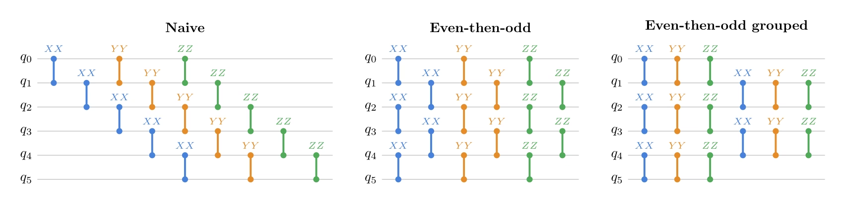
Uspořádání Hamiltoniánu také ovlivňuje Trotterovu chybu. Pokud umístíme nekomutující členy vedle sebe, dochází k přechodům báze častěji, což způsobuje větší Trotterovu chybu. Seskupením členů, které vyžadují stejnou transformaci Pauliho báze, se lze vyhnout redundantním změnám báze.

Zde porovnání používá největší dobu vývoje, která se vyskytuje v odhadech Krylova prvního řádku, $t_{\max} = (r-1)\Delta t,$ pomocí stejné podmínky transpilace.

Pro měření Trotterovy chyby používáme process infidelity mezi trotterizovaným obvodem a přesným vývojem Hamiltoniánu,

$$\begin{equation*} \text{Infidelity}(U,V) = 1-F(U,V) = 1 - \frac{|\operatorname{Tr}(U^\dagger V)|^2}{d^2}, \end{equation*}$$

where $d=2^n$ is the dimension of the Hilbert space.

Tato diagnostika používá husté matice, takže je vhodná pro tento malý 12-qubitový příklad, ale není zamýšlena jako škálovatelná podrutina.

# The comparison uses the largest time that appears in the first-row Krylov estimates.
# Circuit depth does not depend on this numeric value, but the Trotter error does.
comparison_time = (krylov_dim - 1) * dt

def make_heisenberg_hamiltonian_ordered(
    num_qubits: int,
    ordering: str,
    coupling: float = 1.0,
) -> SparsePauliOp:
    """Return the same Heisenberg Hamiltonian with a specified term ordering."""
    terms: list[tuple[str, complex]] = []
    even_edges = [(q, q + 1) for q in range(0, num_qubits - 1, 2)]
    odd_edges = [(q, q + 1) for q in range(1, num_qubits - 1, 2)]

    def append_term(q0: int, q1: int, pauli: str):
        label = ["I"] * num_qubits
        label[num_qubits - 1 - q0] = pauli[0]
        label[num_qubits - 1 - q1] = pauli[1]
        terms.append(("".join(label), coupling))

    if ordering == "naive":
        for pauli in ("XX", "YY", "ZZ"):
            for q in range(num_qubits - 1):
                append_term(q, q + 1, pauli)
    elif ordering == "even-then-odd":
        for pauli in ("XX", "YY", "ZZ"):
            for q0, q1 in even_edges + odd_edges:
                append_term(q0, q1, pauli)
    elif ordering == "even-odd edge-grouped":
        for q0, q1 in even_edges + odd_edges:
            for pauli in ("XX", "YY", "ZZ"):
                append_term(q0, q1, pauli)
    else:
        raise ValueError(f"Unknown ordering: {ordering}")

    return SparsePauliOp.from_list(terms).simplify()

def build_numeric_evolution_circuit(
    hamiltonian: SparsePauliOp,
    synthesis,
    time_value: float,
    **synthesis_kwargs,
) -> QuantumCircuit:
    """Build a numeric circuit for exp(-i H t) with a chosen synthesis rule."""
    evolution_gate = PauliEvolutionGate(
        hamiltonian,
        time=time_value,
        synthesis=synthesis(**synthesis_kwargs),
    )
    circuit = QuantumCircuit(hamiltonian.num_qubits)
    circuit.append(evolution_gate, range(hamiltonian.num_qubits))
    return circuit

def process_infidelity(
    circuit: QuantumCircuit,
    exact_matrix: np.ndarray,
) -> float:
    """Return 1 - |Tr(U_circuit† U_exact) / d|²."""
    circuit_matrix = np.asarray(Operator(circuit).data)
    dim = circuit_matrix.shape[0]
    normalized_trace = np.vdot(circuit_matrix, exact_matrix) / dim
    fidelity = np.abs(normalized_trace) ** 2
    return float(np.clip(1.0 - fidelity, 0.0, 1.0))

hamiltonians_by_ordering = {
    ordering: make_heisenberg_hamiltonian_ordered(
        num_qubits, ordering, coupling=1.0
    )
    for ordering in ["naive", "even-then-odd", "even-odd edge-grouped"]
}

print(f"Comparison time: {comparison_time}\n")

for order_name, ham_ordered in hamiltonians_by_ordering.items():
    print(f"{order_name}:")
    print([op for op, _ in ham_ordered.to_list()])
    print()

print("Precomputing the exact evolution operator... ", end="")
exact_matrix = la.expm(-1j * comparison_time * hamiltonian.to_matrix())
print("Done")

Comparison time: 0.8567979964335799

naive:
['IIIIIIIIIIXX', 'IIIIIIIIIXXI', 'IIIIIIIIXXII', 'IIIIIIIXXIII', 'IIIIIIXXIIII', 'IIIIIXXIIIII', 'IIIIXXIIIIII', 'IIIXXIIIIIII', 'IIXXIIIIIIII', 'IXXIIIIIIIII', 'XXIIIIIIIIII', 'IIIIIIIIIIYY', 'IIIIIIIIIYYI', 'IIIIIIIIYYII', 'IIIIIIIYYIII', 'IIIIIIYYIIII', 'IIIIIYYIIIII', 'IIIIYYIIIIII', 'IIIYYIIIIIII', 'IIYYIIIIIIII', 'IYYIIIIIIIII', 'YYIIIIIIIIII', 'IIIIIIIIIIZZ', 'IIIIIIIIIZZI', 'IIIIIIIIZZII', 'IIIIIIIZZIII', 'IIIIIIZZIIII', 'IIIIIZZIIIII', 'IIIIZZIIIIII', 'IIIZZIIIIIII', 'IIZZIIIIIIII', 'IZZIIIIIIIII', 'ZZIIIIIIIIII']

even-then-odd:
['IIIIIIIIIIXX', 'IIIIIIIIXXII', 'IIIIIIXXIIII', 'IIIIXXIIIIII', 'IIXXIIIIIIII', 'XXIIIIIIIIII', 'IIIIIIIIIXXI', 'IIIIIIIXXIII', 'IIIIIXXIIIII', 'IIIXXIIIIIII', 'IXXIIIIIIIII', 'IIIIIIIIIIYY', 'IIIIIIIIYYII', 'IIIIIIYYIIII', 'IIIIYYIIIIII', 'IIYYIIIIIIII', 'YYIIIIIIIIII', 'IIIIIIIIIYYI', 'IIIIIIIYYIII', 'IIIIIYYIIIII', 'IIIYYIIIIIII', 'IYYIIIIIIIII', 'IIIIIIIIIIZZ', 'IIIIIIIIZZII', 'IIIIIIZZIIII', 'IIIIZZIIIIII', 'IIZZIIIIIIII', 'ZZIIIIIIIIII', 'IIIIIIIIIZZI', 'IIIIIIIZZIII', 'IIIIIZZIIIII', 'IIIZZIIIIIII', 'IZZIIIIIIIII']

even-odd edge-grouped:
['IIIIIIIIIIXX', 'IIIIIIIIIIYY', 'IIIIIIIIIIZZ', 'IIIIIIIIXXII', 'IIIIIIIIYYII', 'IIIIIIIIZZII', 'IIIIIIXXIIII', 'IIIIIIYYIIII', 'IIIIIIZZIIII', 'IIIIXXIIIIII', 'IIIIYYIIIIII', 'IIIIZZIIIIII', 'IIXXIIIIIIII', 'IIYYIIIIIIII', 'IIZZIIIIIIII', 'XXIIIIIIIIII', 'YYIIIIIIIIII', 'ZZIIIIIIIIII', 'IIIIIIIIIXXI', 'IIIIIIIIIYYI', 'IIIIIIIIIZZI', 'IIIIIIIXXIII', 'IIIIIIIYYIII', 'IIIIIIIZZIII', 'IIIIIXXIIIII', 'IIIIIYYIIIII', 'IIIIIZZIIIII', 'IIIXXIIIIIII', 'IIIYYIIIIIII', 'IIIZZIIIIIII', 'IXXIIIIIIIII', 'IYYIIIIIIIII', 'IZZIIIIIIIII']

Precomputing the exact evolution operator... Done

Nejprve udržujeme pravidlo syntézy pevně nastavené na jeden Trotterův krok prvního řádu a měníme pouze uspořádání Pauliho členů. Cílem tohoto porovnání je především zjistit, jak moc lze snížit hloubku obvodu a náklady na dvouqubitové brány odhalením disjunktních hran mezi nejbližšími sousedy transpileru.

ordering_comparison_rows = []
infidelity_reps = [1, 2, 4, 8]

for ordering, ham_ordered in hamiltonians_by_ordering.items():
    for reps in infidelity_reps:
        circuit = build_numeric_evolution_circuit(
            ham_ordered,
            LieTrotter,
            comparison_time,
            reps=reps,
        )
        decomposed_circuit = simple_transpilation(circuit)
        infidelity = process_infidelity(decomposed_circuit, exact_matrix)
        ordering_comparison_rows.append(
            {
                "ordering": ordering,
                "synthesis": f"LieTrotter(reps={reps})",
                "infidelity": infidelity,
                **summarize_circuit(decomposed_circuit),
            }
        )
        if reps == 1:
            print(f"Circuit for {ordering} ordering:")
            print([op for op, _ in ham_ordered.to_list()])
            display(decomposed_circuit.draw("mpl", fold=-1, scale=0.6))

ordering_comparison_df = pd.DataFrame(ordering_comparison_rows)
display(ordering_comparison_df)

hamiltonian_for_synthesis = hamiltonians_by_ordering["even-odd edge-grouped"]

Circuit for naive ordering:
['IIIIIIIIIIXX', 'IIIIIIIIIXXI', 'IIIIIIIIXXII', 'IIIIIIIXXIII', 'IIIIIIXXIIII', 'IIIIIXXIIIII', 'IIIIXXIIIIII', 'IIIXXIIIIIII', 'IIXXIIIIIIII', 'IXXIIIIIIIII', 'XXIIIIIIIIII', 'IIIIIIIIIIYY', 'IIIIIIIIIYYI', 'IIIIIIIIYYII', 'IIIIIIIYYIII', 'IIIIIIYYIIII', 'IIIIIYYIIIII', 'IIIIYYIIIIII', 'IIIYYIIIIIII', 'IIYYIIIIIIII', 'IYYIIIIIIIII', 'YYIIIIIIIIII', 'IIIIIIIIIIZZ', 'IIIIIIIIIZZI', 'IIIIIIIIZZII', 'IIIIIIIZZIII', 'IIIIIIZZIIII', 'IIIIIZZIIIII', 'IIIIZZIIIIII', 'IIIZZIIIIIII', 'IIZZIIIIIIII', 'IZZIIIIIIIII', 'ZZIIIIIIIIII']

Circuit for even-then-odd ordering:
['IIIIIIIIIIXX', 'IIIIIIIIXXII', 'IIIIIIXXIIII', 'IIIIXXIIIIII', 'IIXXIIIIIIII', 'XXIIIIIIIIII', 'IIIIIIIIIXXI', 'IIIIIIIXXIII', 'IIIIIXXIIIII', 'IIIXXIIIIIII', 'IXXIIIIIIIII', 'IIIIIIIIIIYY', 'IIIIIIIIYYII', 'IIIIIIYYIIII', 'IIIIYYIIIIII', 'IIYYIIIIIIII', 'YYIIIIIIIIII', 'IIIIIIIIIYYI', 'IIIIIIIYYIII', 'IIIIIYYIIIII', 'IIIYYIIIIIII', 'IYYIIIIIIIII', 'IIIIIIIIIIZZ', 'IIIIIIIIZZII', 'IIIIIIZZIIII', 'IIIIZZIIIIII', 'IIZZIIIIIIII', 'ZZIIIIIIIIII', 'IIIIIIIIIZZI', 'IIIIIIIZZIII', 'IIIIIZZIIIII', 'IIIZZIIIIIII', 'IZZIIIIIIIII']

Circuit for even-odd edge-grouped ordering:
['IIIIIIIIIIXX', 'IIIIIIIIIIYY', 'IIIIIIIIIIZZ', 'IIIIIIIIXXII', 'IIIIIIIIYYII', 'IIIIIIIIZZII', 'IIIIIIXXIIII', 'IIIIIIYYIIII', 'IIIIIIZZIIII', 'IIIIXXIIIIII', 'IIIIYYIIIIII', 'IIIIZZIIIIII', 'IIXXIIIIIIII', 'IIYYIIIIIIII', 'IIZZIIIIIIII', 'XXIIIIIIIIII', 'YYIIIIIIIIII', 'ZZIIIIIIIIII', 'IIIIIIIIIXXI', 'IIIIIIIIIYYI', 'IIIIIIIIIZZI', 'IIIIIIIXXIII', 'IIIIIIIYYIII', 'IIIIIIIZZIII', 'IIIIIXXIIIII', 'IIIIIYYIIIII', 'IIIIIZZIIIII', 'IIIXXIIIIIII', 'IIIYYIIIIIII', 'IIIZZIIIIIII', 'IXXIIIIIIIII', 'IYYIIIIIIIII', 'IZZIIIIIIIII']

ordering           synthesis  infidelity  depth  size  \
0                   naive  LieTrotter(reps=1)    0.999917     15    33   
1                   naive  LieTrotter(reps=2)    0.805998     21    66   
2                   naive  LieTrotter(reps=4)    0.271389     33   132   
3                   naive  LieTrotter(reps=8)    0.074590     57   264   
4           even-then-odd  LieTrotter(reps=1)    0.999917      6    33   
5           even-then-odd  LieTrotter(reps=2)    0.805998     12    66   
6           even-then-odd  LieTrotter(reps=4)    0.271389     24   132   
7           even-then-odd  LieTrotter(reps=8)    0.074590     48   264   
8   even-odd edge-grouped  LieTrotter(reps=1)    0.998432      6    33   
9   even-odd edge-grouped  LieTrotter(reps=2)    0.653843     12    66   
10  even-odd edge-grouped  LieTrotter(reps=4)    0.181529     24   132   
11  even-odd edge-grouped  LieTrotter(reps=8)    0.045244     48   264   

    2q gates  2q depth  
0         33        15  
1         66        21  
2        132        33  
3        264        57  
4         33         6  
5         66        12  
6        132        24  
7        264        48  
8         33         6  
9         66        12  
10       132        24  
11       264        48

Při reps=1 pozorujeme, že uspořádání sudé-pak-liché i sudo-liché seskupené podle hran obě sníží hloubku z 15 na 6 odhalením paralelních dvouqubitových vrstev, zatímco počet dvouqubitových bran zůstává stejný u všech tří uspořádání. Všechna tři uspořádání však mají infidelity blízkou 1, takže procházíme počet opakování Trotterova kroku, abychom uspořádání jasněji odlišili. Se zvyšujícím se počtem opakování klesá infidelity uspořádání even-odd edge-grouped rychleji než u ostatních dvou a dosahuje 0,045 při reps=8 oproti 0,075 pro naivní a sudé-pak-liché uspořádání.

Porovnání syntézy produktového vzorce

Dále prozkoumáme různá pokročilá nastavení trotterizace, s fixním uspořádáním Hamiltoniánu na sudo-liché seskupené podle hran. Uvažujeme Lie-Trotter prvního řádu, Suzuki-Trotter druhého řádu a Suzuki-Trotter čtvrtého řádu.

synthesis_comparison_rows = []

for num_trotter_steps in [1, 2, 3, 4, 5]:
    synthesis_cases = [
        ("LieTrotter", LieTrotter, {"reps": num_trotter_steps}),
        (
            "SuzukiTrotter(order=2)",
            SuzukiTrotter,
            {"order": 2, "reps": num_trotter_steps},
        ),
        (
            "SuzukiTrotter(order=4)",
            SuzukiTrotter,
            {"order": 4, "reps": num_trotter_steps},
        ),
    ]
    for label, synthesis, kwargs in synthesis_cases:
        circuit = build_numeric_evolution_circuit(
            hamiltonian_for_synthesis,
            synthesis,
            comparison_time,
            **kwargs,
        )
        decomposed_circuit = simple_transpilation(circuit)
        synthesis_comparison_rows.append(
            {
                "synthesis": label,
                "reps": kwargs["reps"],
                "infidelity": process_infidelity(
                    decomposed_circuit, exact_matrix
                ),
                **summarize_circuit(decomposed_circuit),
            }
        )

synthesis_comparison_df = pd.DataFrame(synthesis_comparison_rows)
display(synthesis_comparison_df.sort_values(["2q gates", "2q depth"]))

# For memory free
exact_matrix = None

synthesis  reps    infidelity  depth  size  2q gates  \
0               LieTrotter     1  9.984324e-01      6    33        33   
1   SuzukiTrotter(order=2)     1  9.733399e-01      9    51        51   
3               LieTrotter     2  6.538427e-01     12    66        66   
4   SuzukiTrotter(order=2)     2  2.522533e-01     15    84        84   
6               LieTrotter     3  3.197242e-01     18    99        99   
7   SuzukiTrotter(order=2)     3  4.804050e-02     21   117       117   
9               LieTrotter     4  1.815291e-01     24   132       132   
10  SuzukiTrotter(order=2)     4  1.453103e-02     27   150       150   
12              LieTrotter     5  1.161770e-01     30   165       165   
2   SuzukiTrotter(order=4)     1  2.884402e-01     33   183       183   
13  SuzukiTrotter(order=2)     5  5.803455e-03     33   183       183   
5   SuzukiTrotter(order=4)     2  1.641162e-03     63   348       348   
8   SuzukiTrotter(order=4)     3  2.907076e-05     93   513       513   
11  SuzukiTrotter(order=4)     4  2.791061e-06    123   678       678   
14  SuzukiTrotter(order=4)     5  4.736685e-07    153   843       843   

    2q depth  
0          6  
1          9  
3         12  
4         15  
6         18  
7         21  
9         24  
10        27  
12        30  
2         33  
13        33  
5         63  
8         93  
11       123  
14       153

Lie-Trotter dává nejmělčí obvod, ale má největší chybu, zatímco Suzuki-Trotter čtvrtého řádu je přesnější, ale zvyšuje hloubku obvodu. Pro zbytek tutoriálu volíme Suzuki-Trotter druhého řádu, protože poskytuje obvod s malou hloubkou při podstatném snížení Trotterovy chyby vzhledem ke vzorci prvního řádu.

Odstranění řízené brány časového vývoje

V rozšířeném swap testu vyžaduje řízení časového vývoje jedním ancilla qubitem, aby ancilla řídila mnoho bran napříč systémem. To může způsobit značnou režii při směrování a v nejhorším případě efektivně vyžaduje konektivitu typu all-to-one. Aby se tomu předešlo, je možná další optimalizace nahrazením řízené brány časového vývoje verzí bez řízení, s využitím symetrie Hamiltoniánu. Podívejme se na následující obvod.

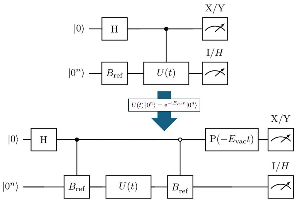
Zde $B_{\rm ref}$ připravuje referenční stav, $B_{\rm ref}|0^n\rangle = |\psi_{0}\rangle$.

Místo nejprve připravit $\frac{1}{\sqrt{2}}(|0\rangle+|1\rangle)|\psi_0\rangle$ a poté aplikovat $U(t)$ pouze na větev $|1\rangle$, obvod přímo připraví obě větve jako

$$\begin{equation*} |0\rangle|\psi_0\rangle \quad \text{and} \quad |1\rangle|\psi_d\rangle , \end{equation*}$$

where

$$\begin{equation*} |\psi_d\rangle = U(d\Delta t)|\psi_0\rangle . \end{equation*}$$

Obvod nejprve aplikuje Hadamardovu bránu na ancillu a připraví referenční stav pouze na větvi $|1\rangle$:

$$\begin{equation*} |0\rangle |0^n\rangle \longrightarrow \frac{|0\rangle |0^n\rangle + |1\rangle B_{\rm ref}|0^n\rangle}{\sqrt{2}} = \frac{|0\rangle |0^n\rangle + |1\rangle |\psi_0\rangle}{\sqrt{2}} . \end{equation*}$$

Poté je neřízený operátor časového vývoje aplikován na obě větve:

$$\begin{equation*} \frac{|0\rangle |0^n\rangle + |1\rangle |\psi_0\rangle}{\sqrt{2}} \longrightarrow \frac{|0\rangle U(t)|0^n\rangle + |1\rangle U(t)|\psi_0\rangle}{\sqrt{2}} . \end{equation*}$$

Protože Hamiltonián zachovává počet excitací, vidíme, že $|0^n\rangle$ je jeho vlastním stavem, a tedy vývojový operátor akumuluje pouze fázi podle Hamiltoniánu:

$$\begin{equation*} U(t)|0^n\rangle = e^{-iE_{\rm vac}t}|0^n\rangle . \end{equation*}$$

Therefore,

$$\begin{equation*} \frac{|0\rangle U(t)|0^n\rangle + |1\rangle U(t)|\psi_0\rangle}{\sqrt{2}} = \frac{e^{-iE_{\rm vac}t}|0\rangle |0^n\rangle + |1\rangle U(t)|\psi_0\rangle}{\sqrt{2}} . \end{equation*}$$

Dále je $B_{\rm ref}$ aplikován pouze na větev $|0\rangle$.

$$\begin{equation*} \frac{e^{-iE_{\rm vac}t}|0\rangle |\psi_0\rangle + |1\rangle U(t)|\psi_0\rangle}{\sqrt{2}} . \end{equation*}$$

V tomto okamžiku mají obě větve dodatečnou relativní fázi. Abychom ji odstranili, aplikujeme fázovou bránu na ancillu

$$\begin{equation*} P(-E_{\rm vac}t) = \begin{pmatrix} 1 & 0 \\ 0 & e^{-iE_{\rm vac}t} \end{pmatrix}. \end{equation*}$$

Toto transformuje stav jako

$$\begin{equation*} \frac{e^{-iE_{\rm vac}t}|0\rangle |\psi_0\rangle + |1\rangle U(t)|\psi_0\rangle}{\sqrt{2}} \longrightarrow \frac{e^{-iE_{\rm vac}t}|0\rangle |\psi_0\rangle + e^{-iE_{\rm vac}t}|1\rangle U(t)|\psi_0\rangle}{\sqrt{2}} . \end{equation*}$$

Tedy, až na irelevantní globální fázi, jsme konečně připravili

$$\begin{equation*} |\Phi_{0d}\rangle = \frac{ |0\rangle|\psi_0\rangle + |1\rangle U(t)|\psi_0\rangle }{\sqrt{2}} . \end{equation*}$$

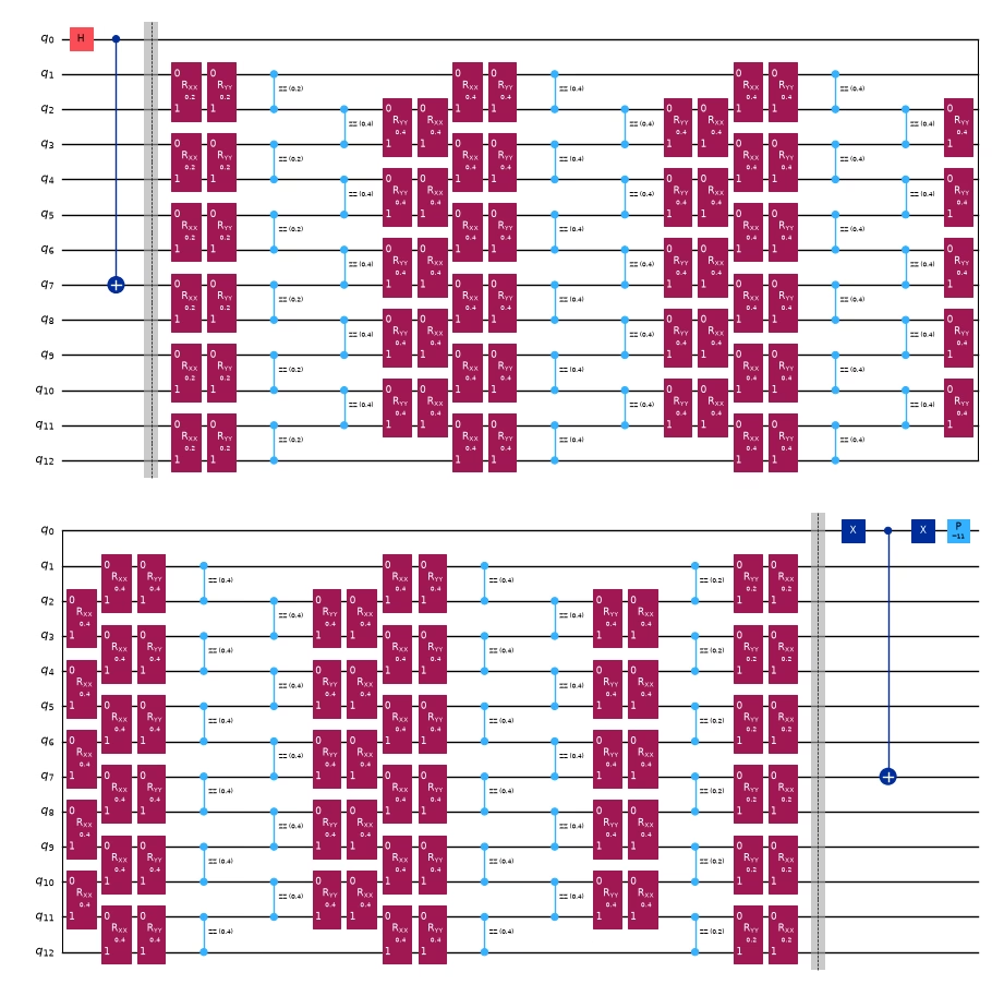
V dalším bloku kódu implementujeme tento obvod bez řízení.

controlled_extended_swap_test = extended_swap_test

# Reuse the ordering and synthesis rule selected by the comparison above.
evol_gate_optimized = PauliEvolutionGate(
    hamiltonian_for_synthesis,
    time=t,
    synthesis=SuzukiTrotter(order=2, reps=num_trotter_steps),
)

uncontrolled_evolution = QuantumCircuit(num_qubits, name="U_ST2(t)")
uncontrolled_evolution.append(evol_gate_optimized, range(num_qubits))

controlled_state_prep = QuantumCircuit(num_qubits + 1, name="C-Prep")
for q, bit in enumerate(reversed(ref_bitstring)):
    if bit == "1":
        controlled_state_prep.cx(ancilla, system_qubits[q])

vacuum_bitstring = "0" * num_qubits
vacuum_energy = basis_state_expectation_sparse(hamiltonian, "0" * num_qubits)

optimized_extended_swap_test = QuantumCircuit(num_qubits + 1)
optimized_extended_swap_test.h(ancilla)

# Prepare |psi_ref> only on the |1> branch.
optimized_extended_swap_test.compose(controlled_state_prep, inplace=True)
optimized_extended_swap_test.barrier()

# Apply the Trotterized time evolution without control.
optimized_extended_swap_test.compose(
    uncontrolled_evolution,
    qubits=system_qubits,
    inplace=True,
)
optimized_extended_swap_test.barrier()

# Map |0>|0...0> to |0>|psi_ref>, leaving the |1> branch unchanged.
optimized_extended_swap_test.x(ancilla)
optimized_extended_swap_test.compose(controlled_state_prep, inplace=True)
optimized_extended_swap_test.x(ancilla)

# Cancel the known vacuum phase so that the same X/Y observables can be used.
optimized_extended_swap_test.p(-vacuum_energy * t, ancilla)
optimized_extended_swap_test = simple_transpilation(
    optimized_extended_swap_test
)

print(f"Vacuum energy E_vac = {vacuum_energy:.1f}")
display(
    optimized_extended_swap_test.assign_parameters({t: 1.0}).draw(
        "mpl", scale=0.5, fold=26
    )
)

Vacuum energy E_vac = 11.0+0.0j

Transpilace

Nyní transpilujeme řízené a neřízené obvody, aby byly spustitelné na hardwaru. Porovnejme výsledek transpilovaných obvodů.

pass_manager = generate_preset_pass_manager(
    backend=backend,
    optimization_level=3,
)

isa_controlled_extended_swap_test = pass_manager.run(
    controlled_extended_swap_test
)

pass_manager = generate_preset_pass_manager(
    backend=backend, optimization_level=3, routing_method="none"
)
isa_optimized_extended_swap_test = pass_manager.run(
    optimized_extended_swap_test
)

transpilation_result = [
    {
        "label": "abstract controlled U(t)",
        **summarize_circuit(isa_controlled_extended_swap_test),
    },
    {
        "label": "optimized non-controlled U(t)",
        **summarize_circuit(isa_optimized_extended_swap_test),
    },
]

display(pd.DataFrame(transpilation_result))

def filter_qubits_from_layout(layout):
    q_layout = Layout(
        {
            physical: virtual
            for physical, virtual in layout.get_physical_bits().items()
            if virtual._register.name == "q"
        }
    )
    return q_layout

print(
    filter_qubits_from_layout(
        isa_optimized_extended_swap_test.layout.initial_layout
    )
)

isa_observables = [
    op.apply_layout(isa_optimized_extended_swap_test.layout)
    for op in observables
]

label  depth   size  2q gates  2q depth
0       abstract controlled U(t)  15457  23786      4686      4580
1  optimized non-controlled U(t)    261   1716       307        57

Layout({
18: <Qubit register=(13, "q"), index=0>,
5: <Qubit register=(13, "q"), index=1>,
6: <Qubit register=(13, "q"), index=2>,
7: <Qubit register=(13, "q"), index=3>,
8: <Qubit register=(13, "q"), index=4>,
9: <Qubit register=(13, "q"), index=5>,
10: <Qubit register=(13, "q"), index=6>,
11: <Qubit register=(13, "q"), index=7>,
12: <Qubit register=(13, "q"), index=8>,
13: <Qubit register=(13, "q"), index=9>,
14: <Qubit register=(13, "q"), index=10>,
15: <Qubit register=(13, "q"), index=11>,
19: <Qubit register=(13, "q"), index=12>
})

Krok 3: Spuštění pomocí Qiskit primitiv

Dalším krokem je odeslat stejný parametrizovaný obvod pro několik hodnot $d$. Pro každé $d$ odhadneme čtyři očekávané hodnoty: $X\otimes I$, $Y\otimes I$, $X\otimes (H-T)$ a $Y\otimes (H-T)$. Tyto čtyři čísla jsou poté zkombinovány do komplexních prvků prvního řádku $\mathcal{S}_{0d}$ a $\mathcal{H}_{0d}$.

Zde $\mathcal{S}_{00}=1$ a $\mathcal{H}_{00}=\langle\psi_{0}|(H-T)|\psi_{0}\rangle=\langle\psi_{0}|H|\psi_{0}\rangle-\tau$ lze vypočítat klasicky, protože $\lvert\psi_0\rangle$ je řídký, takže případ $d=0$ přeskočíme.

pub_list = []
d_values = list(range(1, krylov_dim))

# Exact local statevector estimator.
estimator = StatevectorEstimator()

# We use the circuit before the transpilation for the local simulator,
# but we will use the transpiled circuit for the real backend.
for d in d_values:
    parameter_values = [d * dt]

    for ob in observables:
        pub_list.append(
            (
                optimized_extended_swap_test,
                ob,
                parameter_values,
            )
        )

job = estimator.run(pub_list)

# Local PrimitiveJob does not provide Runtime-style job inputs,
# so preserve the inputs directly.
inputs = pub_list
result = job.result()

print(f"Number of Krylov basis states: r = {len(d_values)}")
print(f"Number of PUBs: {len(pub_list)}")
print(f"Each d uses observables: {observable_labels}")

Number of Krylov basis states: r = 9
Number of PUBs: 36
Each d uses observables: ['Re S_0d', 'Im S_0d', 'Re shifted H_0d', 'Im shifted H_0d']

Krok 4: Následné zpracování a vrácení výsledku v požadovaném klasickém formátu

Po odhadu projektovaných matic regularizujeme a řešíme GEVP

$$\begin{equation*} \mathcal{H}\mathbf{c} = E\mathcal{S}\mathbf{c}. \end{equation*}$$

Nejmenší zobecněné vlastní číslo dává odhad KQD energie základního stavu.

h_shifted_row_est = np.zeros(krylov_dim, dtype=complex)
s_row_est = np.zeros(krylov_dim, dtype=complex)

h_shifted_row_est[0] = ref_energy - shift_tau
s_row_est[0] = 1.0

for idx, (pub_input, pub_result) in enumerate(zip(inputs, result)):
    d_index, obs_index = divmod(idx, len(observables))
    ev = np.asarray(pub_result.data.evs).reshape(-1)[0]
    std = np.asarray(pub_result.data.stds).reshape(-1)[0]

    if obs_index == 0:
        s_row_est[d_index + 1] = ev
    elif obs_index == 1:
        s_row_est[d_index + 1] += 1j * ev
    elif obs_index == 2:
        h_shifted_row_est[d_index + 1] = ev
    elif obs_index == 3:
        h_shifted_row_est[d_index + 1] += 1j * ev

# H_0d = shifted_H_0d + tau * S_0d.
h_row_est = h_shifted_row_est + shift_tau * s_row_est

h_matrix_est = la.toeplitz(h_row_est.conj(), h_row_est)
s_matrix_est = la.toeplitz(s_row_est.conj(), s_row_est)

s_eigvals = la.eigvalsh(0.5 * (s_matrix_est + s_matrix_est.conj().T))
positive_s_eigvals = s_eigvals[s_eigvals > 1e-12]
s_condition_number = (
    positive_s_eigvals[-1] / positive_s_eigvals[0]
    if len(positive_s_eigvals) > 0
    else np.inf
)

with np.printoptions(precision=3, suppress=True):
    print("Estimated first row of S:")
    print(s_row_est)
    print()
    print("Estimated first row of H:")
    print(h_row_est)
    print()
    print("Eigenvalues of the estimated overlap matrix S:")
    print(s_eigvals)
    print(f"Condition number above 1e-12: {s_condition_number:.3e}")
    print()

Estimated first row of S:
[ 1.   +0.j     0.758-0.596j  0.203-0.836j -0.291-0.636j -0.444-0.229j
 -0.276+0.053j -0.044+0.051j  0.006-0.121j -0.155-0.218j -0.345-0.101j]

Estimated first row of H:
[ 7.   +0.j     4.842-4.76j   0.044-6.185j -3.791-3.653j -4.137+0.39j
 -1.495+2.654j  1.331+1.777j  1.85 -0.763j -0.032-2.278j -2.222-1.372j]

Eigenvalues of the estimated overlap matrix S:
[-0.     0.     0.     0.     0.     0.     0.01   0.355  3.526  6.109]
Condition number above 1e-12: 1.904e+12

Nyní vyřešíme zobecněný problém vlastních čísel pomocí matic rekonstruovaných z odhadů obvodu. V ideálním statevector výpočtu s přesným vývojem v reálném čase by to mělo reprodukovat přesný projektovaný výsledek. V praxi mohou odchylky pocházet z trotterizace, chyby vzorkování a numerické nestability matice překryvu.

Pozorujeme, jak energie konverguje se zvyšující se dimenzí Krylovova podprostoru.

exact_evals = diagonalize_single_1_subspace(hamiltonian)
exact_ground = min(exact_evals)
print("exact ground state energy:  ", exact_ground)

threshold = 1e-12
energy_convergence = []

for r in range(1, krylov_dim + 1):
    energy_est_kqd, coeffs_est, retained_est = solve_thresholded_gevp(
        h_matrix_est[:r, :r],
        s_matrix_est[:r, :r],
        threshold=threshold,
    )
    energy_convergence.append(energy_est_kqd)
    print(
        f"Krylov ground state energy (dim={r}, retained={retained_est}): ",
        energy_est_kqd,
    )

exact ground state energy:   3.136296694843727
Krylov ground state energy (dim=1, retained=1):  7.0
Krylov ground state energy (dim=2, retained=2):  4.184510657551266
Krylov ground state energy (dim=3, retained=3):  3.5539074630394136
Krylov ground state energy (dim=4, retained=4):  3.3366270761341044
Krylov ground state energy (dim=5, retained=5):  3.252017453225087
Krylov ground state energy (dim=6, retained=6):  3.2300275138879186
Krylov ground state energy (dim=7, retained=7):  3.2299154099085685
Krylov ground state energy (dim=8, retained=7):  3.2298063744216776
Krylov ground state energy (dim=9, retained=7):  3.2296778282872456
Krylov ground state energy (dim=10, retained=8):  3.223647515867734

def plot_energy_convergence(energy_convergence, exact_ground, krylov_dim):
    fig, ax = plt.subplots(figsize=(7, 4.5))

    ax.plot(
        range(1, krylov_dim + 1),
        energy_convergence,
        marker="o",
        label="KQD estimate",
    )

    ax.axhline(
        exact_ground,
        linestyle="--",
        label=f"Exact ground energy = {exact_ground:.6f}",
    )

    ax.set_xlabel("Krylov dimension")
    ax.set_ylabel("Ground-state energy")
    ax.grid(True, alpha=0.3)
    ax.legend()
    plt.tight_layout()
    plt.show()

plot_energy_convergence(energy_convergence, exact_ground, krylov_dim)

Příklad hardwaru ve velkém měřítku

Předchozí sekce používala 12-qubitový model, aby bylo možné použít statevector simulaci jako diagnostiku. Nyní stejný workflow KQD škálujeme na 30-qubitový Heisenbergův řetězec a připravujeme workload pro spuštění na hardwaru IBM Quantum.

Kroky 1-4 sloučené do jediného bloku kódu

Zde nyní spojíme všechny tyto detaily do jediného workflow ve větším měřítku, který je poté spuštěn na našem reálném kvantovém hardwaru. V této sekci aplikujeme realistická nastavení pro zmírnění chyb, abychom zlepšili spolehlivost výsledků. Protože prvky matice odpovídající různým hodnotám $d$ lze vyhodnotit paralelně, používáme režim Batch pro jejich efektivní spuštění.

# -------------------------Step 1-------------------------

# Map the classical problem to quantum circuits and observables.
# Problem and KQD parameters.
large_num_qubits = 30
large_krylov_dim = 7
large_num_trotter_steps = 3
large_dt = np.pi / (3 * (large_num_qubits - 1))
large_t = Parameter("t_large")

# Use a single excitation near the center of the chain.
large_excitation_qubit = large_num_qubits // 2
large_ref_label = ["0"] * large_num_qubits
large_ref_label[large_num_qubits - 1 - large_excitation_qubit] = "1"
large_ref_bitstring = "".join(large_ref_label)

# Use the ordering and product formula selected in the preceding section.
large_hamiltonian = make_heisenberg_hamiltonian_ordered(
    large_num_qubits,
    ordering="even-odd edge-grouped",
    coupling=1.0,
)
large_ref_energy = float(
    np.real(
        basis_state_expectation_sparse(large_hamiltonian, large_ref_bitstring)
    )
)
large_vacuum_energy = float(
    np.real(
        basis_state_expectation_sparse(
            large_hamiltonian, "0" * large_num_qubits
        )
    )
)

large_evolution_gate = PauliEvolutionGate(
    large_hamiltonian,
    time=large_t,
    synthesis=SuzukiTrotter(order=2, reps=large_num_trotter_steps),
)
large_uncontrolled_evolution = QuantumCircuit(
    large_num_qubits,
    name="U_ST2_large(t)",
)
large_uncontrolled_evolution.append(
    large_evolution_gate,
    range(large_num_qubits),
)

# Build the control-free extended-swap-test circuit.
large_ancilla = 0
large_system_qubits = list(range(1, large_num_qubits + 1))

large_controlled_state_prep = QuantumCircuit(
    large_num_qubits + 1,
    name="C-Prep-large",
)
large_controlled_state_prep.cx(
    large_ancilla,
    large_system_qubits[large_excitation_qubit],
)

large_extended_swap_test = QuantumCircuit(large_num_qubits + 1)
large_extended_swap_test.h(large_ancilla)
large_extended_swap_test.compose(large_controlled_state_prep, inplace=True)
large_extended_swap_test.compose(
    large_uncontrolled_evolution,
    qubits=large_system_qubits,
    inplace=True,
)
large_extended_swap_test.x(large_ancilla)
large_extended_swap_test.compose(
    large_controlled_state_prep.inverse(),
    inplace=True,
)
large_extended_swap_test.x(large_ancilla)
large_extended_swap_test.p(
    -large_vacuum_energy * large_t,
    large_ancilla,
)

# Reuse the Hamiltonian-shifting construction from the preceding section.
(
    large_obs_x_shifted_hamiltonian,
    large_obs_y_shifted_hamiltonian,
    large_shift_tau,
) = make_reduced_heisenberg_observables(large_ref_bitstring)

large_observables = [
    SparsePauliOp("I" * large_num_qubits + "X"),
    SparsePauliOp("I" * large_num_qubits + "Y"),
    large_obs_x_shifted_hamiltonian,
    large_obs_y_shifted_hamiltonian,
]
large_observable_labels = [
    "Re S_0d",
    "Im S_0d",
    "Re shifted H_0d",
    "Im shifted H_0d",
]

# -------------------------Step 2-------------------------

# Optimize the problem for quantum execution.
# Select a real backend and transpile the parameterized circuit to ISA form.
large_backend = service.backend("ibm_boston")
large_pass_manager = generate_preset_pass_manager(
    backend=large_backend, optimization_level=3, routing_method="none"
)
large_isa_circuit = large_pass_manager.run(large_extended_swap_test)
large_isa_observables = [
    observable.apply_layout(large_isa_circuit.layout)
    for observable in large_observables
]

large_two_qubit_gate_count = sum(
    instruction.operation.num_qubits == 2
    for instruction in large_isa_circuit.data
)

print(f"Backend: {large_backend.name}")
print(f"System qubits: {large_num_qubits}")
print(f"Total circuit qubits: {large_isa_circuit.num_qubits}")
print(f"Krylov dimension: {large_krylov_dim}")
print(f"Time step: {large_dt:.6f}")
print(f"Shift tau: {large_shift_tau}")
print(f"ISA circuit depth: {large_isa_circuit.depth()}")
print(f"ISA two-qubit gates: {large_two_qubit_gate_count}")
print(
    f"ISA two-qubit depth: {large_isa_circuit.depth(lambda x: x[0].num_qubits == 2)}"
)

# -------------------------Step 3-------------------------

# Execute on quantum hardware with Qiskit Runtime primitives.
# Submit one job per d, with all four observables in that job.
large_d_values = list(range(1, large_krylov_dim))
retrieve_batch_id = None
large_jobs = []

if retrieve_batch_id is None:
    large_estimator_options = {
        "default_shots": 8192,
        "dynamical_decoupling": {
            "enable": True,
            "sequence_type": "XpXm",
        },
        "resilience": {
            "measure_mitigation": True,
            "measure_noise_learning": {
                "num_randomizations": 32,
                "shots_per_randomization": 256,
            },
            "layer_noise_learning": {
                "max_layers_to_learn": 4,
                "layer_pair_depths": [0, 1, 2, 4, 16, 32],
                "num_randomizations": 32,
                "shots_per_randomization": 128,
            },
            "zne_mitigation": True,
            "zne": {
                "amplifier": "pea",
                "noise_factors": [1.0, 1.5, 2.0],
                "extrapolator": ("exponential", "linear"),
            },
        },
        "twirling": {
            "enable_gates": True,
            "enable_measure": True,
            "num_randomizations": 32,
            "shots_per_randomization": 256,
            "strategy": "active-accum",
        },
    }

    with Batch(backend=large_backend) as large_batch:
        large_batch_id = large_batch.session_id
        large_estimator = EstimatorV2(
            mode=large_batch,
            options=large_estimator_options,
        )
        # Krylov quantum diagonalization of lattice Hamiltonians -> TUT_KQDOLH.
        large_estimator.options.environment.job_tags = ["TUT_KQDOLH"]

        for d in large_d_values:
            parameter_values = [d * large_dt]
            pubs_for_d = [
                (large_isa_circuit, observable, parameter_values)
                for observable in large_isa_observables
            ]
            job = large_estimator.run(pubs_for_d)
            large_jobs.append(job)
            print(
                f"Submitted d={d}: job_id={job.job_id()}, "
                f"PUBs={len(pubs_for_d)}"
            )

    print(f"Batch ID: {large_batch_id}")
else:
    large_batch_id = retrieve_batch_id
    large_jobs = service.jobs(
        session_id=large_batch_id,
        limit=None,
        descending=False,
    )

large_job_ids_by_d = {
    d: job.job_id() for d, job in zip(large_d_values, large_jobs)
}
print(f"Job IDs by d: {large_job_ids_by_d}")

# -------------------------Step 4-------------------------

# Post-process the quantum results and solve the classical GEVP.
# Reconstruct the first rows of S and the shifted Hamiltonian matrix.
large_s_row_est = np.zeros(large_krylov_dim, dtype=complex)
large_h_shifted_row_est = np.zeros(large_krylov_dim, dtype=complex)
large_s_row_est[0] = 1.0
large_h_shifted_row_est[0] = large_ref_energy - large_shift_tau

for d, job in zip(large_d_values, large_jobs):
    job_result = job.result()

    if len(job_result) != len(large_observables):
        raise RuntimeError(
            f"Expected {len(large_observables)} PUB results for d={d}, "
            f"but received {len(job_result)}."
        )

    expectation_values = [
        np.asarray(pub_result.data.evs).reshape(-1)[0]
        for pub_result in job_result
    ]

    large_s_row_est[d] = expectation_values[0] + 1j * expectation_values[1]
    large_h_shifted_row_est[d] = (
        expectation_values[2] + 1j * expectation_values[3]
    )

# H_0d = shifted_H_0d + tau * S_0d.
large_h_row_est = large_h_shifted_row_est + large_shift_tau * large_s_row_est

large_s_matrix_est = la.toeplitz(
    large_s_row_est.conj(),
    large_s_row_est,
)
large_h_matrix_est = la.toeplitz(
    large_h_row_est.conj(),
    large_h_row_est,
)

large_exact_gnd = min(diagonalize_single_1_subspace(large_hamiltonian))

large_energy_convergence = []

with np.printoptions(precision=5, suppress=True):
    print("Estimated first row of S:")
    print(large_s_row_est)
    print("Estimated first row of H:")
    print(large_h_row_est)
    print("exact ground state energy:  ", large_exact_gnd)

    for r in range(1, large_krylov_dim + 1):
        energy_est_kqd, coeffs_est, retained_est = solve_thresholded_gevp(
            large_h_matrix_est[:r, :r],
            large_s_matrix_est[:r, :r],
            threshold=5e-2,
        )
        large_energy_convergence.append(energy_est_kqd)
        print(
            f"Krylov ground state energy (dim={r}, retained={retained_est}): ",
            energy_est_kqd,
        )

plot_energy_convergence(
    large_energy_convergence, large_exact_gnd, large_krylov_dim
)

Backend: ibm_boston
System qubits: 30
Total circuit qubits: 156
Krylov dimension: 7
Time step: 0.036110
Shift tau: 25.0
ISA circuit depth: 219
ISA two-qubit gates: 728
ISA two-qubit depth: 52
Job IDs by d: {1: 'd9fl4p4jeosc73fk4dg0', 2: 'd9fl4pineu4c739poecg', 3: 'd9fl4q2neu4c739poedg', 4: 'd9fl4qhhtsac739fjgn0', 5: 'd9fl4r4jeosc73fk4dhg', 6: 'd9fl4rkjeosc73fk4dj0'}
Estimated first row of S:
[ 1.     +0.j       0.42055-0.65466j -0.17883-0.73125j -0.64523-0.31601j
 -0.70781+0.55574j -0.02467+0.70525j  0.59301+0.55602j]
Estimated first row of H:
[ 25.      +0.j       10.3419 -16.5586j   -5.017  -18.03933j
 -16.44797 -6.98173j -17.17081+14.84502j   0.62722+17.81196j
  15.68886+12.74875j]
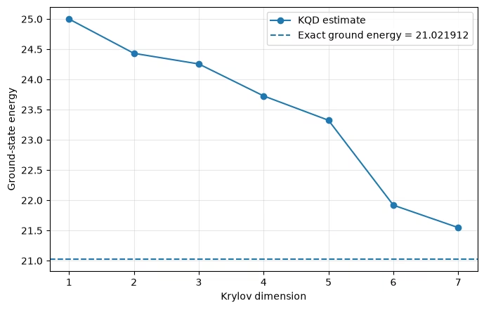
exact ground state energy:   21.021912418526902
Krylov ground state energy (dim=1, retained=1):  25.0
Krylov ground state energy (dim=2, retained=2):  24.432409110686205
Krylov ground state energy (dim=3, retained=3):  24.256856893278556
Krylov ground state energy (dim=4, retained=4):  23.727409826799715
Krylov ground state energy (dim=5, retained=4):  23.324720470780864
Krylov ground state energy (dim=6, retained=5):  21.91957579005085
Krylov ground state energy (dim=7, retained=5):  21.548331214122644

Příloha: Pohled na funkci Hamiltoniánu (spektrální filtr)

Hlavní workflow prezentoval KQD operačně: sestavit Krylovovu bázi ze stavů vyvinutých v reálném čase, odhadnout projektované matice $\mathcal{H}$ a $\mathcal{S}$ a vyřešit GEVP. Tato příloha se vrací ke stejnému výpočtu z komplementárního úhlu, který vysvětluje proč KQD funguje: pohled na funkci Hamiltoniánu, neboli spektrální filtr [3], [5]. Znovu využívá 12-qubitový model, časový krok $\Delta t$ a Krylovovo řešení již získané výše; není vyžadováno žádné nové spuštění obvodu.

Referenční stav jako energetické rozdělení

Nechť Hamiltonián má vlastní rozklad

$$\begin{equation*} H=\sum_{m} E_m\,|E_m\rangle\!\langle E_m|, \qquad E_0\le E_1\le\cdots, \end{equation*}$$

s energetickými vlastními stavy $|E_m\rangle$. Každý referenční stav lze rozvinout v této vlastní bázi,

$$\begin{equation*} |\psi_{0}\rangle=\sum_m a_m\,|E_m\rangle, \qquad a_m=\langle E_m|\psi_{0}\rangle, \end{equation*}$$

nese tedy spektrální váhu $p_m=|a_m|^2$ při každé energii $E_m$. Referenční energie je střední hodnotou tohoto rozdělení, $\langle H\rangle_{0}=\sum_m p_m E_m$.

Vlastní rozklad obecného $n$-qubitového Hamiltoniánu je exponenciálně nákladný, takže tento pohled slouží pouze jako diagnostika, která není součástí algoritmu. Zde ho však můžeme levně spočítat pro stejný problém s $n=12$: Heisenbergův Hamiltonián zachovává celkový počet excitací a referenční stav $|000001000000\rangle$ nese jedinou excitaci, takže celý jeho spektrální obsah leží v podprostoru jedné excitace, jehož dimenze roste pouze lineárně s $n$. Proto znovu použijeme přesný blok jedné excitace (již dříve použitý jako benchmark) a vyčteme referenční rozdělení $\{(E_m, p_m)\}$ uvnitř tohoto podprostoru.

# Exact single-excitation-subspace decomposition of the reference state.
# This reuses make_heisenberg_hamiltonian / _basis_state_transition_amplitude_sparse
# and the n=12 `hamiltonian` and `ref_bitstring` defined in the small-scale example.
single_excitation_states = [1 << k for k in range(num_qubits)]

h_single = np.array(
    [
        [
            _basis_state_transition_amplitude_sparse(hamiltonian, bra, ket)
            for ket in single_excitation_states
        ]
        for bra in single_excitation_states
    ]
)
h_single = 0.5 * (h_single + h_single.conj().T)

subspace_evals, subspace_evecs = la.eigh(h_single)
subspace_evals = np.real(subspace_evals)

# Reference-state coordinates inside the single-excitation subspace.
ref_position = single_excitation_states.index(int(ref_bitstring, 2))
ref_in_subspace = np.zeros(num_qubits, dtype=complex)
ref_in_subspace[ref_position] = 1.0

# Amplitudes and spectral weights of the reference in the energy eigenbasis.
ref_eigen_amplitudes = subspace_evecs.conj().T @ ref_in_subspace
ref_spectral_weights = np.abs(ref_eigen_amplitudes) ** 2

print(f"Single-excitation subspace dimension: {num_qubits}")
print(f"Subspace ground-state energy:         {subspace_evals[0]:.6f}")
print(
    f"Reference energy (sum p_m E_m):       {np.sum(ref_spectral_weights * subspace_evals):.6f}"
)
print(f"Reference weight on subspace ground:  {ref_spectral_weights[0]:.6f}")

Single-excitation subspace dimension: 12
Subspace ground-state energy:         3.136297
Reference energy (sum p_m E_m):       7.000000
Reference weight on subspace ground:  0.163827

KQD se učí filtr, který přetváří toto rozdělení

Hamiltoniánská funkce $f(H)$ je definována pomocí spektrálního počtu,

$$\begin{equation*} f(H)=\sum_m f(E_m)\,|E_m\rangle\!\langle E_m|, \end{equation*}$$

neboli jinými slovy, vážený součet vlastních projektorů. Její aplikace na referenční stav přetváří každou spektrální amplitudu, $a_m \to a_m f(E_m)$:

$$\begin{equation*} f(H)\,|\psi_{0}\rangle=\sum_m a_m\,f(E_m)\,|E_m\rangle . \end{equation*}$$

Kdyby $f$ byla ostře koncentrovaná na nejnižší energii ($f(E_0)=1$ a jinak $f(E_m)\approx 0$), pak by $f(H)$ fungovala jako projektor na základní stav a normalizovaný výstup by byl (blízko) základnímu stavu. Proto je dobrý dolnopropustný spektrální filtr v energii přesně to, co chceme.

KQD nepředepisuje $f$ předem. Místo toho rozvíjí filtr v bázi reálné časové evoluce,

$$\begin{equation*} f_{\rm KQD}(E)=\sum_{\ell=0}^{r-1} c_\ell\, e^{-i\ell\Delta t E}, \end{equation*}$$

trigonometrickou funkci energie, jejíž koeficienty $\{c_\ell\}$ jsou přesně vlastním vektorem GEVP vyřešeným výše. Minimalizace Rayleighova podílu $\mathbf{c}^\dagger\mathcal{H}\mathbf{c}/\mathbf{c}^\dagger\mathcal{S}\mathbf{c}$ je tedy totéž jako učení se filtru, který nejlépe potlačuje váhu excitovaných stavů v referenčním stavu. Větší Krylovova dimenze $r$ dává filtru více stupňů volnosti a ostřejší vrchol v energii základního stavu.

Pomocná funkce níže vyhodnocuje tento naučený filtr na energetické ose; poté ho aplikujeme na referenční rozdělení získané výše.

def trigonometric_krylov_filter(
    coeffs: np.ndarray,
    energies: np.ndarray,
    time_step: float,
) -> np.ndarray:
    """Evaluate the learned Krylov filter f(E) = sum_l c_l exp(-i l dt E)."""
    values = np.zeros_like(energies, dtype=complex)
    for ell, coeff in enumerate(coeffs):
        values += coeff * np.exp(-1j * ell * time_step * energies)
    return values

def filtered_spectral_weights(
    weights: np.ndarray,
    filter_values: np.ndarray,
) -> np.ndarray:
    """Reshape spectral weights by |f(E)|^2 and renormalize."""
    reshaped = weights * np.abs(filter_values) ** 2
    return reshaped / np.sum(reshaped)

# Recover the KQD coefficients from the already-estimated projected matrices.
# The shift only moves H by tau * S, so it does not change the GEVP eigenvector;
# we solve at the full Krylov dimension used in the small-scale example.
_, kqd_coeffs, _ = solve_thresholded_gevp(
    h_matrix_est,
    s_matrix_est,
    threshold=1e-12,
)

filter_on_spectrum = trigonometric_krylov_filter(
    kqd_coeffs, subspace_evals, dt
)
filtered_weights = filtered_spectral_weights(
    ref_spectral_weights, filter_on_spectrum
)

print(f"Ground-state overlap  (reference): {ref_spectral_weights[0]:.4f}")
print(f"Ground-state overlap  (filtered):  {filtered_weights[0]:.4f}")
print(
    f"Mean energy           (reference): {np.sum(ref_spectral_weights * subspace_evals):.6f}"
)
print(
    f"Mean energy           (filtered):  {np.sum(filtered_weights * subspace_evals):.6f}"
)

Ground-state overlap  (reference): 0.1638
Ground-state overlap  (filtered):  0.9638
Mean energy           (reference): 7.000000
Mean energy           (filtered):  3.164503

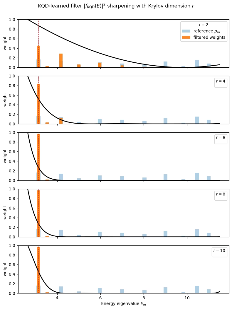
Vizualizace filtru a jeho flexibility

Nejprve ukážeme naučený filtr při plné Krylovově dimenzi použité výše, poté sledujeme, jak se zaostřuje s růstem dimenze $r$.

Sloupce ukazují referenční spektrální váhy $p_m$ (před) a filtrované váhy $p_m|f_{\rm KQD}(E_m)|^2$ (po), spolu s intenzitou naučeného filtru $|f_{\rm KQD}(E)|^2$ na spojité energetické ose. Filtr soustřeďuje váhu na nejnižší energii podprostoru jedné excitace — stejnou energii, ke které konvergoval odhad KQD v malém příkladu. Všimni si, že se jedná o základní stav v rámci sektoru jedné excitace, což je relevantní cíl pro tento referenční stav zachovávající excitace, nikoli globální základní stav.

fig, ax = plt.subplots(figsize=(8, 4))

visible = (ref_spectral_weights > 1e-4) | (filtered_weights > 1e-4)
ax.bar(
    subspace_evals[visible],
    ref_spectral_weights[visible],
    width=0.18,
    alpha=0.45,
    label="reference $p_m$",
)
ax.bar(
    subspace_evals[visible],
    filtered_weights[visible],
    width=0.14,
    alpha=0.9,
    label=r"filtered $p_m\,|f_{\rm KQD}(E_m)|^2$",
)

energy_grid = np.linspace(
    subspace_evals.min() - 0.5, subspace_evals.max() + 0.5, 800
)
filter_intensity = (
    np.abs(trigonometric_krylov_filter(kqd_coeffs, energy_grid, dt)) ** 2
)
filter_intensity /= filter_intensity.max()
ax.plot(
    energy_grid,
    filter_intensity,
    color="k",
    linewidth=2,
    label=r"$|f_{\rm KQD}(E)|^2$ (normalized)",
)

ax.axvline(
    subspace_evals[0],
    color="C3",
    linestyle="--",
    linewidth=1,
    label="subspace ground energy",
)
ax.set_xlabel("Energy eigenvalue $E_m$")
ax.set_ylabel("Spectral weight")
ax.set_ylim(0, 1)
ax.legend(loc="upper right")
plt.tight_layout()
plt.show()

Zvyšování Krylovovy dimenze: flexibilita naučené funkce

Připomeňme, že naučený filtr je trigonometrický polynom v energii s $r$ koeficienty,

$$\begin{equation*} f_{\rm KQD}(E)=\sum_{\ell=0}^{r-1} c_\ell\, e^{-i\ell\Delta t E}. \end{equation*}$$

Krylovova dimenze $r$ je přesně počet volných koeficientů, takže řídí flexibilitu funkce. Malé $r$ může vytvořit pouze široký, pozvolna se měnící filtr, který propouští váhu do nízko položených excitovaných stavů; když se $r$ zvětšuje, filtr může vytvořit užší vrchol při cílové energii a agresivněji potlačit zbývající váhu excitovaných stavů. Toto je spektrálně-filtrový protějšek konvergence energie pozorované v malém příkladu: jak $r$ roste, filtrované rozdělení se soustřeďuje na základní stav podprostoru a odhadovaná energie k němu klesá.

Znovu použijeme již odhadnuté projektované matice výše a jednoduše vyřešíme GEVP pro každý vedoucí blok $r\times r$, poté vyhodnotíme a vykreslíme odpovídající filtr.

# Sweep the Krylov dimension using the leading r x r blocks of the estimated matrices.
sweep_dims = [r for r in (2, 4, 6, 8, krylov_dim) if r <= krylov_dim]
sweep_dims = sorted(set(sweep_dims))

energy_grid = np.linspace(
    subspace_evals.min() - 0.5, subspace_evals.max() + 0.5, 800
)

sweep_cases = []
print(" r    retained    ground overlap    filtered energy")
print("--    --------    --------------    ---------------")
for r in sweep_dims:
    _, coeffs_r, retained_r = solve_thresholded_gevp(
        h_matrix_est[:r, :r],
        s_matrix_est[:r, :r],
        threshold=1e-12,
    )
    filter_on_spectrum_r = trigonometric_krylov_filter(
        coeffs_r, subspace_evals, dt
    )
    filtered_weights_r = filtered_spectral_weights(
        ref_spectral_weights, filter_on_spectrum_r
    )
    filtered_energy_r = float(np.sum(filtered_weights_r * subspace_evals))

    sweep_cases.append((r, coeffs_r, filtered_weights_r))
    print(
        f"{r:2d}    {retained_r:8d}    {filtered_weights_r[0]:14.4f}    {filtered_energy_r:15.6f}"
    )

print(f"\nSubspace ground-state energy (target): {subspace_evals[0]:.6f}")

# One panel per Krylov dimension: filtered spectrum (bars) + filter intensity (curve).
fig, axes = plt.subplots(
    len(sweep_cases),
    1,
    figsize=(8, 2.1 * len(sweep_cases)),
    sharex=True,
)
axes = np.atleast_1d(axes)

for idx, (ax, (r, coeffs_r, filtered_weights_r)) in enumerate(
    zip(axes, sweep_cases)
):
    visible = (ref_spectral_weights > 1e-4) | (filtered_weights_r > 1e-4)
    ax.bar(
        subspace_evals[visible],
        ref_spectral_weights[visible],
        width=0.18,
        alpha=0.35,
        color="C0",
        label="reference $p_m$" if idx == 0 else None,
    )
    ax.bar(
        subspace_evals[visible],
        filtered_weights_r[visible],
        width=0.14,
        alpha=0.9,
        color="C1",
        label="filtered weights" if idx == 0 else None,
    )

    filter_intensity_r = (
        np.abs(trigonometric_krylov_filter(coeffs_r, energy_grid, dt)) ** 2
    )
    filter_intensity_r /= filter_intensity_r.max()
    ax.plot(energy_grid, filter_intensity_r, color="k", linewidth=2)

    ax.axvline(subspace_evals[0], color="C3", linestyle="--", linewidth=1)
    ax.set_ylim(0, 1)
    ax.set_ylabel("weight")
    ax.legend(loc="upper right", title=f"$r={r}$")

axes[-1].set_xlabel("Energy eigenvalue $E_m$")
fig.suptitle(
    r"KQD-learned filter $|f_{\rm KQD}(E)|^2$ sharpening with Krylov dimension $r$",
    y=1.0,
)
fig.tight_layout()
plt.show()

r    retained    ground overlap    filtered energy
--    --------    --------------    ---------------
 2           2            0.4549           4.184510
 4           4            0.8373           3.310168
 6           6            0.9706           3.158100
 8           7            0.9701           3.158725
10           8            0.9638           3.164503

Subspace ground-state energy (target): 3.136297

Další kroky

Pokud tě tato práce zaujala, mohou tě zajímat následující materiály:

Doporučení

• Sample-based Krylov quantum diagonalization of a fermionic lattice model
• Ground-state energy estimation of the Heisenberg chain with VQE
• Quantum diagonalization algorithms course

Reference

[1] E. N. Epperly, L. Lin, and Y. Nakatsukasa, A theory of quantum subspace diagonalization, SIAM Journal on Matrix Analysis and Applications 43, 1263-1290 (2022).

[2] N. Yoshioka, M. Amico, W. Kirby, et al., Diagonalization of large many-body Hamiltonians on a quantum processor, arXiv:2407.14431 (2024).

[3] R. M. Parrish a P. L. McMahon, Quantum filter diagonalization: quantum eigendecomposition without full quantum phase estimation, Physical Review Letters 122, 230401 (2019).

[4] G. Lee, S. Choi, J. Huh a A. F. Izmaylov, Efficient strategies for reducing sampling error in quantum Krylov subspace diagonalization, Digital Discovery 4, 954-969 (2025).

[5] G. Lee, M. Kang, J. Hong, S. Fomichev a J. Huh, Filtered Quantum Phase Estimation, arXiv:2510.04294 (2025).