Pravděpodobnostní eliminace chyb s logickými modely šumu

Odhad doby využití: 28 minut na procesoru Heron r3 (POZNÁMKA: Jedná se pouze o odhad. Vaše skutečná doba běhu se může lišit.)

In this tutorial we will evaluate observables of a 22-site Ising model on a hexagonal lattice using a Heron QPU, which has a heavy-hexagonal qubit topology. Many demonstrations on Heron QPUs focus on systems defined on heavy-hexagonal lattices to match the system's connectivity; however, hexagonal models tend to be more interesting to study as they appear more commonly in nature and are more difficult to simulate classically due to their denser connectivity. Since the qubit topology of the QPU cannot directly support the connectivity of a hexagonal lattice, we must decide how to efficiently embed the hexagonal model onto the qubit topology. In this example we represent each site in the Ising model with a qubit lying on a vertex of the heavy-hex QPU lattice. We use the qubits on the edges (mediator qubits) to facilitate entanglement between the Ising qubits on the vertices. Additionally, the mediator qubits implement entanglement in such a way that they are always expected to return to the ground state $|0\rangle$. If a mediator qubit measures $|1\rangle$, it indicates that a logical error occurred during circuit execution; postselecting only samples with no detected errors on the mediator qubits yields a smaller distribution of logical samples that might have a higher fidelity than the raw, noisy distribution. Not only can we detect that an error occurred by measuring a mediator qubit, we can also determine exactly which logical errors that qubit is capable of detecting throughout the circuit. Removing the noise generators the mediator qubits' symmetry checks are capable of detecting from a noise model leaves a reduced noise model, which can be mitigated using techniques such as probabilistic error cancellation (PEC).

V tomto příkladu notebooku zkombinujeme výše popsanou techniku detekce chyb s PEC, abychom účinněji potlačili kvantový šum, než dokáže kterákoli technika samostatně. Použijeme 49 qubitů k vložení 22qubitového Isingova modelu a dalších 27 mediátorových qubitů použijeme pro detekci chyb. PEC spustíme na postselektovaném šumovém kanálu, abychom potlačili šum, který unikne kontrolám symetrie. Kromě kombinace detekce chyb s PEC použijeme techniky jako je zmírnění chyb čtení pomocí TREX a nemarkovské kontroly chyb, abychom dále potlačili vliv kvantového šumu.

Postup je následující:

1. Klasicky simulovat pozorovatelné střední hodnoty pro 22qubitový hex-Isingův model
2. Implementovat 49qubitový hex-Isingův model detekující chyby pomocí kvantového obvodu a transpilovat na backend QPU
3. Specifikovat provázávací vrstvy v obvodu pomocí samplomatic. Naučíme se a potlačíme šum ovlivňující tyto provázávací vrstvy.
4. Přidat do obvodu nemarkovské kontroly chyb
5. Naučit se šum hradel a čtení ovlivňující obvod
6. Ořezat model šumu o členy detekované kontrolami symetrie
7. Vzorkovat obvod detekující chyby. Postselektovat pouze vzorky, které projdou všemi kontrolami symetrie a nemarkovskými kontrolami chyb, a pro všechny výpočty střední hodnoty použít zmírnění čtení pomocí TREX
   • Vzorkovat obvod detekující chyby
   • Vzorkovat obvod detekující chyby s PEC, ale nepostselektovat na základě kontrol symetrie a potlačit celý naučený šumový kanál.
   • Vzorkovat obvod detekující chyby s PEC. Postselektovat na základě kontrol symetrie a potlačit pouze šum, který je kontrolami nedetekovatelný.
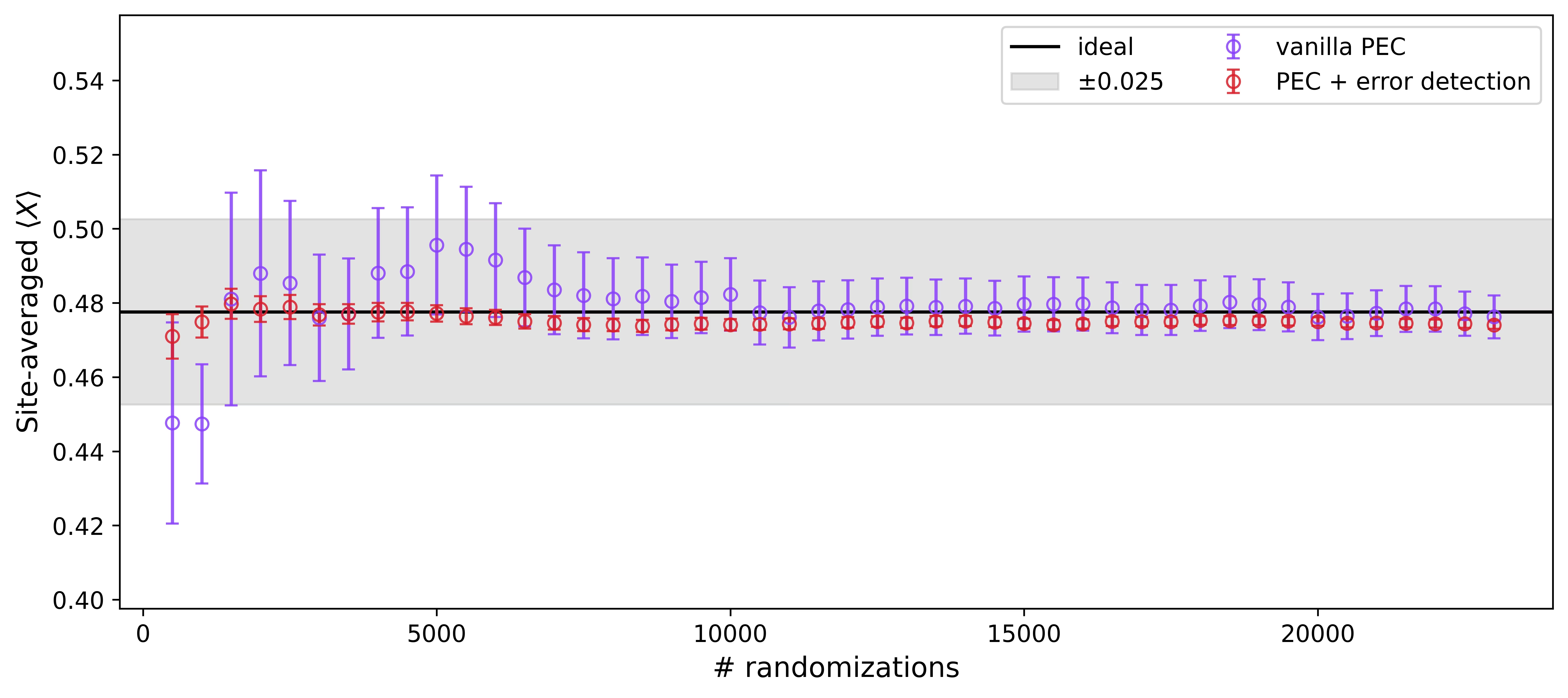
8. Vypočítat střední hodnoty a porovnat strategie. Pozoruj, že QED+PEC účinněji eliminuje šum ovlivňující experiment než kterákoli metoda samostatně a produkuje konvergované střední hodnoty s výrazně méně shoty, než vyžaduje samotné PEC.

Požadavky

Před zahájením tohoto tutoriálu spusťte následující příkaz, abyste získali všechny potřebné balíčky:

%pip install networkx numpy "qiskit[visualization]" "qiskit-ibm-runtime[visualization]" samplomatic qiskit-mitigation matplotlib "qiskit-noise-learning @ git+https://github.com/Qiskit/qiskit-noise-learning.git@ieee-demo-2026" Sbalená buňka níže definuje pomocné funkce pro obrázky používané v celém tomto notebooku.

Kliknutím zobrazíte pomocné funkce pro obrázky

# Added by doQumentation — installs the packages this notebook needs if they are missing
import importlib.util

_needed = {"matplotlib": "matplotlib", "networkx": "networkx", "numpy": "numpy", "qiskit": "qiskit", "qiskit_ibm_runtime": "qiskit-ibm-runtime", "qiskit_mitigation": "qiskit-mitigation", "qiskit_noise_learning": "qiskit-noise-learning@git+https://github.com/Qiskit/qiskit-noise-learning.git@ieee-demo-2026", "samplomatic": "samplomatic"}
_missing = [pip for module, pip in _needed.items()
            if importlib.util.find_spec(module) is None]
# One at a time, so a package that fails to install does not block the others
for _pip in _missing:
    %pip install -q {_pip}
if not _missing:
    print("\u2713 All required packages are installed")

# Figure helpers for this notebook (collapsed): all plotting and styling lives here.
# The chip maps follow the style of Fig. 30 of arXiv:2607.25998.

from math import comb

import matplotlib.pyplot as plt
from matplotlib import cm
from matplotlib.colors import BoundaryNorm
from matplotlib.patches import Circle, Rectangle, Wedge

# one typography scheme for every figure in the notebook
plt.rcParams.update(
    {
        "font.size": 13,
        "axes.titlesize": 15,
        "axes.labelsize": 13,
        "xtick.labelsize": 11,
        "ytick.labelsize": 11,
        "legend.fontsize": 11,
    }
)

def x_labels(layout, n_data):
    """Per-observable tick labels carrying the physical qubit indices (site i = qubit i)."""
    return [f"$X_{{{layout[i]}}}$" for i in range(n_data)]

def plot_layout(backend, layout, n_data):
    """Chip cartoon of the embedding: data qubits green, check qubits orange."""
    from qiskit.visualization import plot_coupling_map

    return plot_coupling_map(
        num_qubits=backend.num_qubits,
        qubit_coordinates=None,
        coupling_map=list(backend.coupling_map.get_edges()),
        figsize=(9, 9),
        qubit_color=[
            "#4CAF50"
            if q in layout[:n_data]
            else "#FF9800"
            if q in layout[n_data:]
            else "#DDDDDD"
            for q in range(backend.num_qubits)
        ],
        qubit_size=220,
        line_width=2,
        font_size=90,
    )

def plot_exact(obs_exact, tick_labels, title):
    plt.figure(figsize=(12, 4))
    plt.plot(obs_exact, "o-")
    plt.title(title)
    plt.xticks(np.arange(len(obs_exact)), tick_labels)
    plt.xlabel("Observable")
    plt.ylabel(r"$\langle X \rangle$")
    plt.grid()

def draw_toy_circuit(
    generate_ed_ising, zz_coeff, x_coeff, include_checks=True
):
    """The boxing pipeline on a 3-plaquette-ring miniature (1 Trotter step) so the box
    structure is legible; every box carries the Twirl / InjectNoise annotations, and with
    ``include_checks`` the terminal xslow non-Markovian error check pattern is appended as in the
    production pipeline."""
    import networkx as nx
    from qiskit.circuit import ClassicalRegister
    from qiskit_mitigation.postselection import XSlowGate
    from samplomatic.transpiler import generate_boxing_pass_manager

    toy, _, _ = generate_ed_ising(nx.cycle_graph(3), 1, zz_coeff, x_coeff)
    toy.add_register(
        ClassicalRegister(3, "data"), ClassicalRegister(3, "check")
    )
    toy.barrier()
    toy.measure(range(3), range(3))
    toy.measure(range(3, 6), range(3, 6))
    toy_boxed = generate_boxing_pass_manager(
        enable_gates=True,
        enable_measures=True,
        inject_noise_targets="gates",
        inject_noise_strategy="individual_modification",
        inject_noise_site="after",
        twirling_strategy="active_circuit",
        measure_annotations="all",
    ).run(toy)
    if include_checks:
        toy_boxed.add_register(
            ClassicalRegister(3, "data_ps"), ClassicalRegister(3, "check_ps")
        )
        toy_boxed.barrier()
        for qb in range(6):
            toy_boxed.append(XSlowGate(), [qb])
        toy_boxed.measure(range(3), toy_boxed.cregs[2])
        toy_boxed.measure(range(3, 6), toy_boxed.cregs[3])
    return toy_boxed.draw("mpl", fold=-1, scale=0.6)

# --- chip-level noise maps ---------------------------------------------------------

BANDS = [1e-5, 2e-5, 3e-5, 4e-5, 6e-5, 1e-4, 2e-4, 3e-4, 4e-4, 6e-4, 1e-3]
CMAP = plt.get_cmap("YlOrBr")
NORM = BoundaryNorm(BANDS, CMAP.N, extend="both")

def _color(rate):
    return (
        "white"
        if rate < BANDS[0]
        else CMAP(NORM(min(rate, BANDS[-1] * 0.999)))
    )

def _layer_sparse(mit, weights):
    """Per-layer labelled terms from the saved run, box-local -> physical qubits."""
    phys = np.sort(mit["layout"])
    return [
        [
            (p, tuple(int(phys[q]) for q in qs if q >= 0), r)
            for p, qs, r in zip(
                mit[f"label_paulis_{i}"],
                mit[f"label_qubits_{i}"],
                w,
                strict=True,
            )
        ]
        for i, w in enumerate(weights)
    ]

def _aggregate(layers):
    """w1[qubit][P] and w2[(a,b)][PaPb]: rates summed over the 3 layers."""
    w1, w2 = {}, {}
    for terms in layers:
        for p, qs, r in terms:
            if len(qs) == 1:
                w1.setdefault(qs[0], dict.fromkeys("XYZ", 0.0))[p] += r
            else:
                (a, pa), (b, pb) = sorted(zip(qs, p, strict=True))
                w2.setdefault(
                    (a, b), {x + y: 0.0 for x in "XYZ" for y in "XYZ"}
                )[pa + pb] += r
    return w1, w2

def draw_noise_map(mit, backend, reduced=False):
    """Chip map of the learned model: X/Y/Z wheel per qubit, 3x3 two-qubit Pauli grid per
    coupler, log-banded colors, dashed outlines for unused hardware.

    With ``reduced=True``, keeps only the error terms the checks cannot see: detectability
    depends on circuit position, so each layer's 0/1 site scales are averaged over its uses.
    """
    from qiskit_ibm_runtime.visualization.embeddings import Embedding

    if reduced:
        scales = [
            mit["site_scales"][mit["site_layer"] == i].mean(axis=0)
            for i in range(3)
        ]
        weights = [mit[f"rates_{i}"] * scales[i] for i in range(3)]
        title = f"Reduced noise model ($\\gamma$ = {mit['gammas'][1]:.1f})"
    else:
        weights = [mit[f"rates_{i}"] for i in range(3)]
        title = f"Full noise model ($\\gamma$ = {mit['gammas'][0]:.0f})"
    w1, w2 = _aggregate(_layer_sparse(mit, weights))

    xy = np.array(
        [(c, -r) for r, c in Embedding.from_backend(backend).coordinates]
    )
    fig, ax = plt.subplots(figsize=(13, 7))
    for a, b in {tuple(sorted(e)) for e in backend.coupling_map.get_edges()}:
        if (
            (
                a,
                b,
            )
            in w2
        ):  # 3x3 Pauli grid laid along the bond (columns: qubit a, rows: qubit b)
            d = xy[b] - xy[a]
            u = d / np.hypot(*d)
            v = np.array([-u[1], u[0]])
            cl, cw = (np.hypot(*d) - 0.6) / 3, 0.17
            for i, Pa in enumerate("XYZ"):
                for j, Pb in enumerate("XYZ"):
                    ax.add_patch(
                        Rectangle(
                            xy[a] + u * (0.3 + i * cl) + v * ((j - 1.5) * cw),
                            cl,
                            cw,
                            angle=np.degrees(np.arctan2(u[1], u[0])),
                            facecolor=_color(w2[a, b][Pa + Pb]),
                            edgecolor="black",
                            lw=0.4,
                            zorder=2,
                        )
                    )
        else:
            ax.plot(
                *zip(xy[a], xy[b], strict=True),
                ls="--",
                lw=0.7,
                color="black",
                alpha=0.5,
                zorder=1,
            )
    for q, (xq, yq) in enumerate(xy):
        if q in w1:  # three-sector wheel: X top, Y lower left, Z lower right
            for P, t0 in (("X", 30), ("Y", 150), ("Z", 270)):
                ax.add_patch(
                    Wedge(
                        (xq, yq),
                        0.3,
                        t0,
                        t0 + 120,
                        facecolor=_color(w1[q][P]),
                        edgecolor="black",
                        lw=0.6,
                        zorder=3,
                    )
                )
            ax.annotate(
                str(q),
                (xq + 0.39, yq - 0.39),
                fontsize=9,
                color="gray",
                ha="left",
                va="top",
                zorder=4,
            )  # southeast, clear of the bond grids
        else:
            ax.add_patch(
                Circle(
                    (xq, yq),
                    0.24,
                    facecolor="none",
                    edgecolor="black",
                    ls="--",
                    lw=0.7,
                    alpha=0.5,
                    zorder=3,
                )
            )
    ux = xy[sorted(w1)]
    ax.set_xlim(ux[:, 0].min() - 2.2, ux[:, 0].max() + 2.2)
    ax.set_ylim(ux[:, 1].min() - 1.6, ux[:, 1].max() + 1.6)
    ax.set_aspect("equal")
    ax.axis("off")
    ax.set_title(title, fontsize=15)
    cb = fig.colorbar(
        cm.ScalarMappable(norm=NORM, cmap=CMAP),
        ax=ax,
        fraction=0.035,
        pad=0.02,
        extend="both",
        ticks=BANDS,
    )
    cb.set_label("coefficient (log bands; white < 1e-05)", fontsize=11)
    cb.ax.set_yticklabels(
        [f"{b:.0e}".replace("e-0", "e-") for b in BANDS], fontsize=10
    )
    _noise_map_legends(fig, ax)

def _noise_map_legends(fig, ax):
    """Weight-1 wheel and weight-2 grid keys, in a reserved band left of the lattice."""
    fig.subplots_adjust(left=0.17)
    axl = ax.inset_axes([-0.185, 0.70, 0.13, 0.24])
    for P, t0 in (("X", 30), ("Y", 150), ("Z", 270)):
        axl.add_patch(
            Wedge(
                (0.5, 0.45),
                0.38,
                t0,
                t0 + 120,
                facecolor="white",
                edgecolor="black",
                lw=0.8,
            )
        )
        axl.annotate(
            P,
            (
                0.5 + 0.2 * np.cos(np.radians(t0 + 60)),
                0.45 + 0.2 * np.sin(np.radians(t0 + 60)),
            ),
            ha="center",
            va="center",
            fontsize=9,
        )
    axl.set_title("weight-1", fontsize=10)
    axl.set_xlim(0, 1)
    axl.set_ylim(0, 1)
    axl.set_aspect("equal")
    axl.axis("off")
    axm = ax.inset_axes([-0.185, 0.32, 0.14, 0.30])
    for i, Pa in enumerate("XYZ"):
        for j, Pb in enumerate("XYZ"):
            axm.add_patch(
                Rectangle(
                    (i / 3, 1 - (j + 1) / 3),
                    1 / 3,
                    1 / 3,
                    facecolor="white",
                    edgecolor="black",
                    lw=0.6,
                )
            )
            axm.annotate(
                Pa + Pb,
                ((i + 0.5) / 3, 1 - (j + 0.5) / 3),
                ha="center",
                va="center",
                fontsize=7.5,
            )
        axm.annotate(Pa, ((i + 0.5) / 3, 1.08), ha="center", fontsize=8.5)
        axm.annotate(
            "XYZ"[i],
            (-0.13, 1 - (i + 0.5) / 3),
            ha="center",
            va="center",
            fontsize=8.5,
        )
    axm.annotate("qubit a", (0.5, 1.27), ha="center", fontsize=9)
    axm.annotate(
        "qubit b", (-0.33, 0.5), rotation=90, va="center", fontsize=9
    )
    axm.set_xlim(-0.35, 1.05)
    axm.set_ylim(-0.05, 1.35)
    axm.set_aspect("equal")
    axm.axis("off")

# --- run diagnostics ---------------------------------------------------------------

def plot_trex(trex_rescale, tick_labels):
    _fig, axt = plt.subplots(figsize=(12, 3))
    axt.stem(np.arange(len(trex_rescale)), (trex_rescale - 1) * 100)
    axt.set_xticks(np.arange(len(trex_rescale)), tick_labels)
    axt.set_xlabel("Observable")
    axt.set_ylabel("Readout correction (%)")
    axt.set_title("TREX rescale factors")
    plt.tight_layout()

def plot_postselection(mit):
    """Accepted shots per PEC randomization against a single binomial at the mean
    acceptance rate: agreement means acceptance is independent of the sampled circuit
    instance, the condition under which pooling accepted shots across randomizations
    is a consistent estimator."""
    _fig, ax = plt.subplots(figsize=(7.5, 3.8))
    counts = mit["acc_counts_post"]
    K, p = 64, counts.mean() / 64
    ks = np.arange(K + 1)
    pmf = np.array([comb(K, k) * p**k * (1 - p) ** (K - k) for k in ks])
    ax.hist(
        counts,
        bins=np.arange(-0.5, K + 1.5),
        density=True,
        alpha=0.6,
        color="#da1e28",
        label="measured",
    )
    ax.plot(ks, pmf, "k-", lw=1.5, label=f"Binomial(64, {p:.3f})")
    ax.set_xlim(-0.5, max(int(counts.max()) + 3, 20))
    ax.set_xlabel("Accepted shots per randomization")
    ax.set_ylabel("Probability")
    ax.legend()
    ax.grid(alpha=0.4)
    plt.tight_layout()

def plot_convergence(mit, obs_exact, n_data):
    """Running site-averaged estimate vs. randomizations for both PEC arms (the S5-consistent
    signed-ratio estimator, evaluated on growing prefixes of the sweep)."""

    def running(prefix):
        bits = np.squeeze(
            np.unpackbits(mit[f"data_{prefix}"], axis=-1)[..., :n_data]
            ^ mit[f"flips_{prefix}"]
        )
        mask = np.squeeze(mit[f"mask_{prefix}"])
        signs = 1 - 2 * (np.squeeze(mit[f"signs_{prefix}"]).sum(axis=-1) % 2)
        qv = (1 - 2 * bits.astype(int)) * mit["trex_rescale"]
        u = (
            (signs[:, None, None] * mask[..., None] * qv)
            .sum(axis=1)
            .mean(axis=1)
        )
        v = signs * mask.sum(axis=1)
        Rs = np.arange(500, len(u) + 1, 500)
        est, err = [], []
        for R in Rs:
            e = u[:R].sum() / v[:R].sum()
            est.append(e)
            err.append(
                np.sqrt(((u[:R] - e * v[:R]) ** 2).sum()) / abs(v[:R].sum())
            )
        return Rs, np.array(est), np.array(err)

    _fig, ax = plt.subplots(figsize=(12, 5))
    ideal_avg = float(np.mean(obs_exact))
    ax.axhline(ideal_avg, color="black", label="ideal")
    ax.fill_between(
        [-400, 24000],
        ideal_avg - 0.025,
        ideal_avg + 0.025,
        color="grey",
        alpha=0.22,
        label=r"$\pm 0.025$",
    )
    for prefix, label, color in (
        ("van", "vanilla PEC", "#8a3ffc"),
        ("post", "PEC + error detection", "#da1e28"),
    ):
        Rs, est, err = running(prefix)
        ax.errorbar(
            Rs,
            est,
            yerr=err,
            marker="o",
            linestyle="",
            markerfacecolor="none",
            color=color,
            alpha=0.85,
            capsize=3,
            label=label,
        )
    ax.set_xlim(-400, 24000)
    ax.set_ylim(ideal_avg - 0.08, ideal_avg + 0.08)
    ax.set_xlabel("# randomizations")
    ax.set_ylabel(r"Site-averaged $\langle X \rangle$")
    ax.legend(ncols=2)

def plot_final(
    obs_exact, baseline, ed, pec, post, gammas, tick_labels, title
):
    """Per-site <X> for every method, with an rms-deviation inset.
    baseline/ed/pec/post are (values, errors) pairs; gammas is (gamma, gamma_post)."""
    x = np.arange(len(obs_exact))
    _fig, ax = plt.subplots(figsize=(13, 5))
    h_ideal = ax.errorbar(
        x, obs_exact, fmt="-", capsize=4, label="ideal", color="black"
    )
    h_base = ax.errorbar(
        x,
        baseline[0],
        yerr=baseline[1],
        fmt=".--",
        capsize=4,
        label="baseline",
        color="#0f62fe",
    )
    h_ed = ax.errorbar(
        x,
        ed[0],
        yerr=ed[1],
        fmt="^",
        capsize=4,
        label="error detection",
        color="#009d9a",
        alpha=0.8,
    )
    h_pec = ax.errorbar(
        x,
        pec[0],
        yerr=pec[1],
        fmt="x",
        capsize=4,
        label=f"PEC ($\\gamma$={gammas[0]:.0f})",
        color="#8a3ffc",
        alpha=0.7,
    )
    h_post = ax.errorbar(
        x,
        post[0],
        yerr=post[1],
        fmt="d",
        capsize=4,
        label=f"PEC + error detection ($\\gamma$={gammas[1]:.0f})",
        color="#da1e28",
    )
    ax.set_xticks(x, tick_labels)
    ax.set_xlabel("Observable")
    ax.set_ylabel("Expectation value")
    # Set the y-axis range using the ideal, baseline, error detection, and PEC + error
    # detection curves, including error bars. Exclude PEC-only values when setting the
    # range so large fluctuations do not make the other curves difficult to distinguish.
    # PEC-only values may fall outside the visible range. Leave room above for the inset.
    series = [np.asarray(obs_exact)] + [
        np.asarray(v) + s * np.asarray(e)
        for v, e in (baseline, ed, post)
        for s in (-1, 1)
    ]
    lo, hi = min(a.min() for a in series), max(a.max() for a in series)
    span = max(hi - lo, 0.1)
    ax.set_ylim(lo - 0.1 * span, hi + 1.05 * span)
    # legend ordered to match the curves' vertical positions in the chart
    ax.legend(
        handles=[h_ideal, h_pec, h_post, h_ed, h_base],
        ncols=5,
        loc="lower center",
        bbox_to_anchor=(0.5, 1.02),
        frameon=False,
    )
    ax.set_title(title, pad=44)

    # inset: rows bottom-to-top so it reads top-to-bottom: PEC, PEC+ED, ED, baseline
    axi = ax.inset_axes([0.36, 0.68, 0.28, 0.26])
    methods = [
        ("baseline", baseline[0], "#0f62fe"),
        ("QED", ed[0], "#009d9a"),
        ("PEC+QED", post[0], "#da1e28"),
        ("PEC", pec[0], "#8a3ffc"),
    ]
    for k, (_nm, vals, color) in enumerate(methods):
        axi.barh(
            k,
            np.sqrt(np.mean((vals - np.array(obs_exact)) ** 2)),
            color=color,
            alpha=0.9,
        )
    axi.set_yticks(range(4), [m[0] for m in methods], fontsize=10)
    axi.set_title("RMS deviation from ideal", fontsize=11)
    axi.tick_params(labelsize=10)
    axi.patch.set_alpha(1.0)
    axi.set_zorder(5)

Klasicky simulujte $\langle X \rangle_i$ pro každé místo v 22qubitovém hex-Isingově modelu

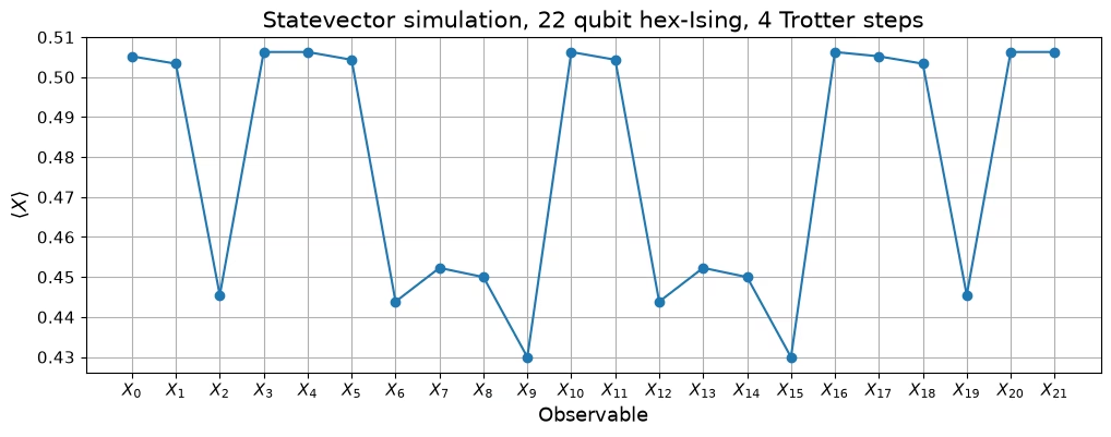
Nejprve použijeme třídu Qiskit Statevector k simulaci přesných cílových hodnot pro náš experiment. Zatímco 22qubitový problém, který řešíme, je klasicky zvládnutelný, simulátor stavového vektoru Qiskit se neškáluje na mnohem větší demonstrace než tato, a pro škálování nad přibližně 50 qubitů bychom potřebovali použít nepřesné simulační techniky, jako je Pauliho propagace. Tento 49qubitový experiment nám umožňuje zkoumat kombinaci detekce chyb se zmírněním chyb ve větším měřítku a zároveň zachovat přístup k ideálním středním hodnotám.

import warnings

import networkx as nx
import numpy as np
from qiskit.circuit import QuantumCircuit
from qiskit.quantum_info import Pauli, Statevector

# Silence two harmless upstream warnings (a Samplomatic default-change notice and a
# numpy datetime timezone notice from the noise-learning circuit generator)
warnings.filterwarnings(
    "ignore", message="The default of the 'inject_noise_site'"
)
warnings.filterwarnings(
    "ignore", message="no explicit representation of timezones"
)

# Hexagonal lattice
data_graph = nx.convert_node_labels_to_integers(
    nx.hexagonal_lattice_graph(2, 3)
)

# Number of Trotter steps and rotation angles
depth = 4
zz_coeff = -np.pi / 4
x_coeff = 3 * np.pi / 8
n_data = data_graph.order()
n_checks = data_graph.size()
n_qubits = n_data + n_checks

qc_data = QuantumCircuit(n_data)
qc_data.h(range(n_data))
for _ in range(depth):
    for edge in data_graph.edges:
        qc_data.rzz(zz_coeff, *edge)
    qc_data.rx(x_coeff, range(n_data))
psi_exact = Statevector(qc_data)

# X on site i = qubit i
observables = ["I" * (n_data - 1 - i) + "X" + "I" * i for i in range(n_data)]
obs_exact = [psi_exact.expectation_value(Pauli(o)).real for o in observables]

plot_exact(
    obs_exact,
    x_labels(range(n_data), n_data),
    f"Statevector simulation, {n_data} qubit hex-Ising, {depth} Trotter steps",
)

Implementujte 49qubitový hex-Isingův model detekující chyby pomocí kvantového obvodu a transpilujte na backend QPU

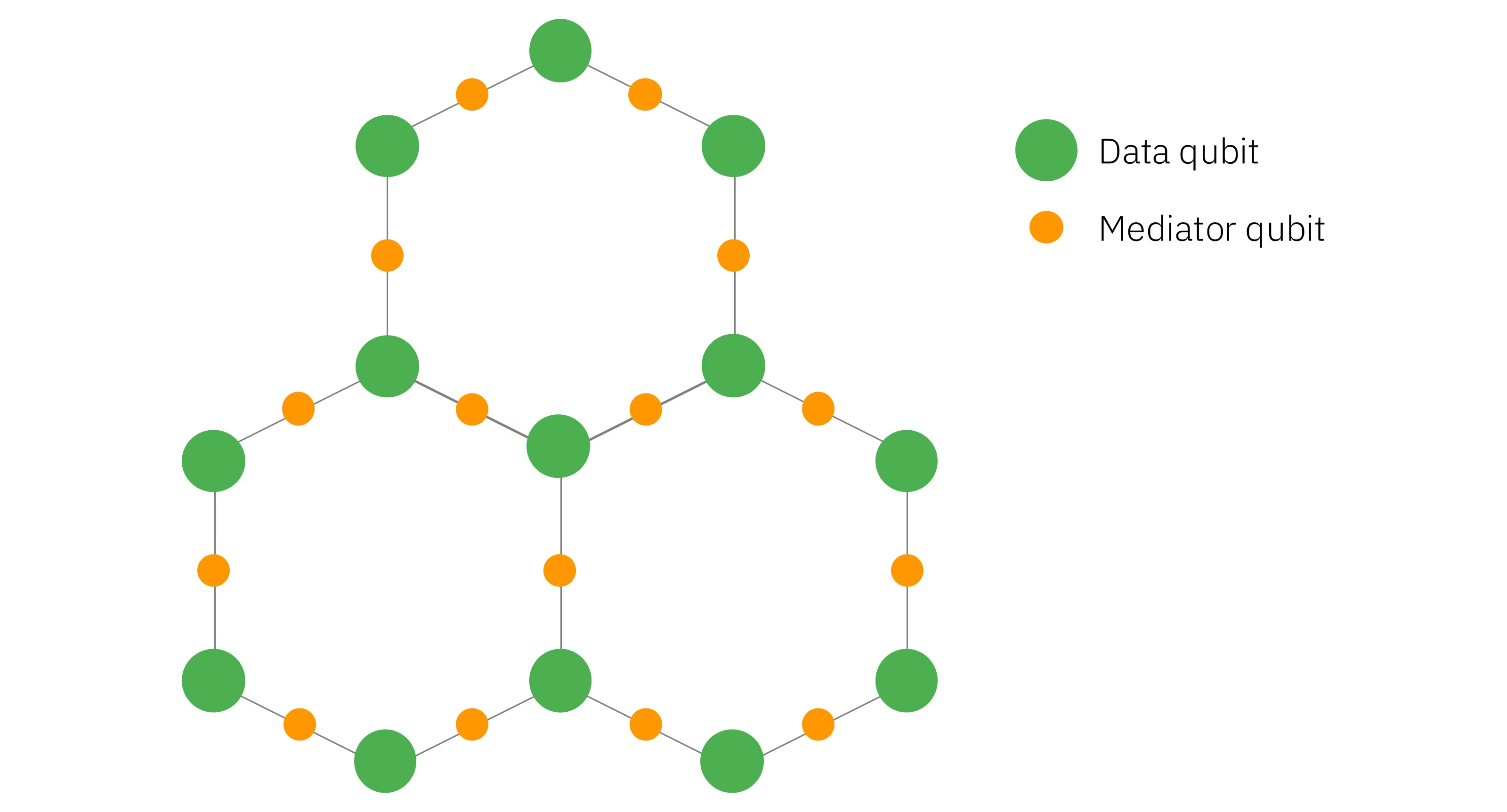
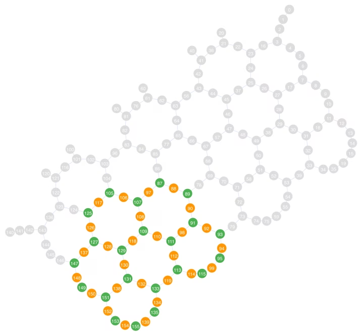
Tento obvod simuluje 4 Trotterovy kroky 22qubitového Isingova Hamiltoniánu s příčným polem na hexagonální mřížce. 22 datových qubitů je vloženo do 49qubitového heavy-hex podgrafu QPU Heron r3, ibm_boston. 27 pomocných (ancilla) qubitů se používá pro dva účely: zprostředkování provázání mezi Isingovými qubity a detekci logických chyb během provádění obvodu. Provázávací vrstvy obvodu jsou implementovány tak, aby se mediátorové qubity před svým závěrečným měřením vrátily do základního stavu $|0\rangle$. Jeden nebo více mediátorových qubitů naměřených ve stavu $|1\rangle$ signalizuje, že vzorek byl poškozen logickou chybou. Vyřazení těchto vzorků může zlepšit věrnost vzorkovaného rozdělení.

Na grafu níže zelené qubity představují 22 Isingových qubitů a oranžové qubity představují 27 mediátorových qubitů.

from qiskit.circuit import ClassicalRegister
from qiskit.transpiler import generate_preset_pass_manager
from qiskit_ibm_runtime import QiskitRuntimeService

backend_name = "ibm_boston"

def generate_ed_ising(graph, depth, zz_coeff, x_coeff):
    """Build the mediated error-detecting Ising circuit for data-qubit `graph`; returns (circuit, CZ layers, hardware graph)."""
    hw_graph = nx.Graph()
    for i, (a, b) in enumerate(graph.edges()):
        hw_graph.add_edges_from(
            [(a, i + graph.order()), (b, i + graph.order())]
        )
    coloring = nx.coloring.greedy_color(
        nx.line_graph(hw_graph), strategy="DSATUR"
    )
    layers_coupling = [
        [e for e, c in coloring.items() if c == i]
        for i in set(coloring.values())
    ]
    circuit = QuantumCircuit(hw_graph.order())
    circuit.h(range(hw_graph.order()))
    for _ in range(depth):
        for angle, qubits in (
            (zz_coeff, range(graph.order(), hw_graph.order())),
            (x_coeff, range(graph.order())),
        ):
            circuit.barrier()
            for layer in layers_coupling:
                for edge in layer:
                    circuit.cz(*edge)
            circuit.barrier()
            circuit.rx(angle, qubits)
    circuit.barrier()
    circuit.h(range(graph.order(), hw_graph.order()))
    return circuit, layers_coupling, hw_graph

service = QiskitRuntimeService()
backend = service.backend(backend_name)

circuit, layers_coupling, hw_graph = generate_ed_ising(
    data_graph, depth, zz_coeff, x_coeff
)

circ_meas = circuit.copy()
data_reg, check_reg = (
    ClassicalRegister(n_data, "data"),
    ClassicalRegister(n_checks, "check"),
)
circ_meas.add_register(data_reg, check_reg)
circ_meas.barrier()
circ_meas.measure(range(n_data), data_reg)
circ_meas.measure(range(n_data, n_qubits), check_reg)

# Physical qubits hosting the 22 Ising sites on ibm_boston, one heavy-hex row per lattice chain;
# the mediator for each edge is the physical qubit sitting between its two data qubits
data_layout = [
    *[95, 93, 91, 89, 87],
    *[115, 113, 111, 109, 107, 105],
    *[135, 133, 131, 129, 127, 125],
    *[155, 153, 151, 149, 147],
]
coupling_graph = nx.Graph(list(backend.coupling_map.get_edges()))
layout = data_layout + [
    next(
        iter(
            nx.common_neighbors(
                coupling_graph, data_layout[a], data_layout[b]
            )
        )
    )
    for a, b in data_graph.edges()
]

circ_trans = generate_preset_pass_manager(
    backend=backend, optimization_level=1, initial_layout=layout
).run(circ_meas)

plot_layout(backend, layout, n_data)

Specifikujte provázávací vrstvy v obvodu pomocí samplomatic.

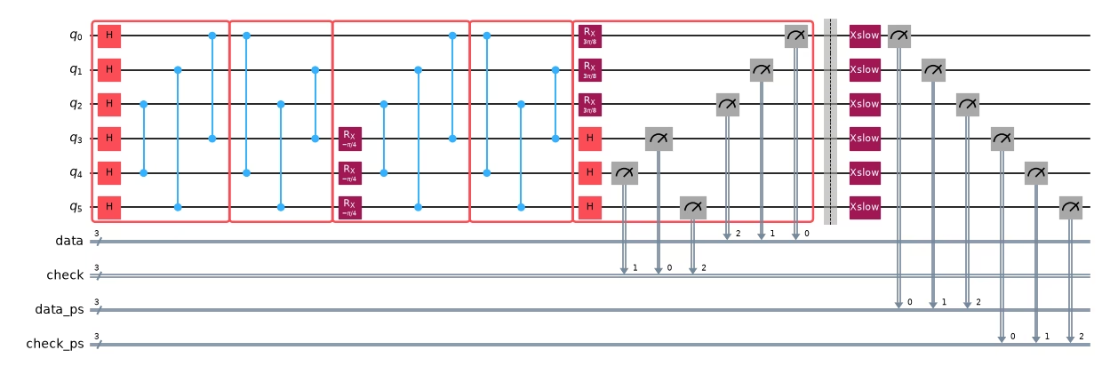
Průchod Samplomatic generate_boxing_pass_manager seskupuje provázávací vrstvy obvodu do anotovaných boxů pro Pauliho twirling a injektáž šumu PEC. Výsledný šablonový obvod a samplex (parametrické rozdělení nad šablonovým obvodem specifikující jeho twirly a injektáž šumu) se používají k definování a provádění všech experimentů učení šumu a vzorkování na QPU. Měřicí boxy nesou také anotaci ChangeBasis, takže rotace, které měří datové qubity v bázi X, jsou dodávány samplexu jako vstup v okamžiku vzorkování namísto toho, aby byly zabudovány přímo do obvodu.

Níže je stejný boxovací průchod aplikován na miniaturní verzi Isingova obvodu detekujícího chyby, abychom mohli vizualizovat strukturu boxovaného obvodu.

from samplomatic.builders import build
from samplomatic.transpiler import generate_boxing_pass_manager
from samplomatic.utils import find_unique_box_instructions

boxed = generate_boxing_pass_manager(
    enable_gates=True,
    enable_measures=True,
    inject_noise_targets="gates",
    inject_noise_strategy="individual_modification",
    inject_noise_site="after",
    twirling_strategy="active_circuit",
    measure_annotations="all",
).run(circ_trans)
template, samplex = build(boxed)
unique_instructions = find_unique_box_instructions(
    boxed, normalize_annotations=None, undress_boxes=True
)

# Measure X on the data qubits and Z on the mediators
basis_key = next(
    s.name
    for s in samplex.inputs().get_specs()
    if s.name.startswith("basis_changes.")
)
meas_basis = np.array(
    [2 if q in set(layout[:n_data]) else 1 for q in sorted(layout)],
    dtype=np.uint8,
)

draw_toy_circuit(generate_ed_ising, zz_coeff, x_coeff, include_checks=False)

Přidejte do obvodu nemarkovské kontroly chyb

Dále do obvodu přidáme nemarkovské kontroly chyb, abychom se chránili proti šumu, který není modelován v našem protokolu učení. Tyto kontroly fungují implementací bitového překlopení dlouhým pulzem a ověřením, že se qubit správně přesunul z jednoho klasického stavu do druhého. Pokud oba qubity na hraně kontrolou neprojdou, je vzorek vyřazen. Nemarkovské kontroly chyb lze použít na začátku nebo na konci obvodu (nebo na obou místech); zde je použijeme pouze na konci. Kontroly také umísťujeme na nevyužité „spektátorové“ (přihlížející) qubity sousedící s obvodem, což poskytuje větší pokrytí proti šumu, který jsou tyto kontroly určeny detekovat.

Pamatujte, že podobně jako kontroly symetrie je i toto formou postselekce, takže musíme zohlednit pokles míry postselekce při kombinaci těchto technik. Konkrétně, pokud $P(\text{nemarkovská chyba}) = \alpha$ a $P(\text{chyba symetrie}) = \beta$, pak potřebujete přibližně $\frac{1}{(1-\alpha)(1-\beta)}$ zašuměných vzorků k získání jednoho logického vzorku.

from qiskit.transpiler import PassManager
from qiskit_mitigation.postselection import PostSelector
from qiskit_mitigation.postselection.passes import (
    AddPostCircuitNonMarkovianErrorChecks,
    AddSpectatorPostCircuitNonMarkovianErrorChecks,
)

add_checks = PassManager(
    [
        AddPostCircuitNonMarkovianErrorChecks(x_pulse_type="xslow"),
        AddSpectatorPostCircuitNonMarkovianErrorChecks(
            backend.coupling_map, x_pulse_type="xslow"
        ),
    ]
)
template_checked = add_checks.run(template)
selector = PostSelector.from_circuit(template_checked, backend.coupling_map)

draw_toy_circuit(generate_ed_ising, zz_coeff, x_coeff, include_checks=True)

Naučte se šum hradel a čtení pro 49qubitový kontrolovaný Isingův obvod

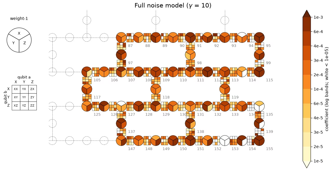
Abychom potlačili šum, musíme namodelovat, jak šum ovlivňuje naše provázávací hradla. Zde se pro každou ze tří jedinečných provázávacích vrstev obvodu naučíme model šumu Pauli-Lindblad pomocí qiskit-noise-learning. Později tento model šumu ořežeme o generátory chyb, které jsou detekovatelné kontrolami symetrie, a pomocí PEC potlačíme pouze zbývající šumový kanál. Mapa níže zobrazuje tři naučené vrstvy na QPU; každý qubit je kolo svých rychlostí X/Y/Z váhy 1 a každá vazba (coupler) je mřížka 3×3 rychlostí Pauliho váhy 2 na daném páru. Hodnota $\gamma$ rovna $10$ implikuje režii vzorkování $\gamma^2=10^2=100$.

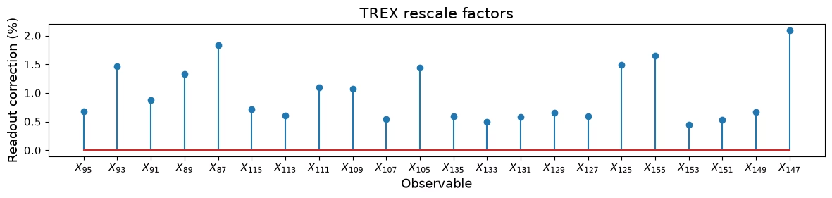
Korekce čtení (TREX) pocházejí přímo ze SPAM cest ve fitu modelu šumu. Stonkový graf pod mapou šumu QPU zobrazuje faktory přeškálování TREX pro jednotlivé pozorovatelné veličiny.

from qiskit.quantum_info import PauliLindbladMap, QubitSparsePauli
from qiskit_ibm_runtime import Executor, Session
from qiskit_ibm_runtime.quantum_program import QuantumProgram
from qiskit_mitigation.trex import TREX
from qiskit_noise_learning.analysis import (
    ComputeObservables,
    CurveFitObservables,
    FlipPostSelect,
    LeastSquaresSolve,
)
from qiskit_noise_learning.circuit_generator import ExecutorCircuitGenerator
from qiskit_noise_learning.experiment_builder import (
    BindFragmentDepths,
    CompleteSequences,
    EvenDepthVanillaPaths,
    Experiment,
    GenerateInstructionSequences,
    IdentifyRelations,
    MergeInstructionSequences,
    SPAMPaths,
    VanillaInstructionSequences,
)
from qiskit_noise_learning.gate_sets import QiskitGateSet
from qiskit_noise_learning.models import PauliLindbladModel
from qiskit_noise_learning.models.utils import split_pauli_lindblad_model
from samplomatic.annotations import InjectNoise
from samplomatic.utils import get_annotation

gate_set = QiskitGateSet(
    target=backend.target,
    qubit_subset=sorted(
        {
            boxed.find_bit(q).index
            for i in unique_instructions
            for q in i.qubits
        }
    ),
)
ref_to_qubits = {}
for inst in unique_instructions:
    if ann := get_annotation(inst.operation, InjectNoise):
        gate_set.add_box_as_gate(inst, name=ann.ref)
        ref_to_qubits[ann.ref] = sorted(
            boxed.find_bit(q).index for q in inst.qubits
        )

fidelity_model = PauliLindbladModel.k_local(
    gate_set, gate_k={**{r: 2 for r in ref_to_qubits}, "M": 1, "P": 1}
)
experiment = (
    EvenDepthVanillaPaths()
    + VanillaInstructionSequences()
    + IdentifyRelations()
    + SPAMPaths()
    + GenerateInstructionSequences()
    + MergeInstructionSequences()
    + CompleteSequences()
    + BindFragmentDepths([2, 4, 8, 12])
).run(Experiment(fidelity_model=fidelity_model, shots=384, randomizations=64))

circuit_generator = ExecutorCircuitGenerator(
    gate_set, pass_manager=add_checks
)
program_learn, data_mapper = circuit_generator.generate(experiment)

session = Session(backend)
executor_options = {"environment": {"job_tags": ["TUT_PECLNM"]}}
fit = circuit_generator.collect(
    Executor(session, options=executor_options).run(program_learn).result(),
    data_mapper,
)
fit = (
    FlipPostSelect()
    + ComputeObservables()
    + CurveFitObservables()
    + LeastSquaresSolve()
).run(fit)
print(
    "learning shots removed by checks:",
    f"{float(fit.raw_data.datatree['0']['data_mask'].mean()):.4f}",
)

# TREX factors from the fit's SPAM paths: the fit only identifies the product of
# state-prep and measurement error, so hand TREX the composition of the two maps
spam = fidelity_model.to_pauli_lindblad_maps(
    fit.model_data, include_spam=True
)
spam_map = spam["P"].compose(spam["M"])
z_terms = [
    QubitSparsePauli(("Z", [layout[i]]), num_qubits=backend.num_qubits)
    for i in range(n_data)
]
trex_rescale = np.array(
    [TREX.calculate_trex_factor(spam_map, z) for z in z_terms]
)

# learned maps come back in backend qubit indexing; samplex wants box-local order
plm = split_pauli_lindblad_model(fit.model).model
noise_maps = {}
for ref, m in plm.to_pauli_lindblad_maps(fit.model_data).items():
    box = ref_to_qubits[ref]
    noise_maps[ref] = PauliLindbladMap.from_sparse_list(
        [
            (p, tuple(box.index(q) for q in qs), r)
            for p, qs, r in m.to_sparse_list()
        ],
        num_qubits=len(box),
    )
# Full-PEC cost: each learned layer acts twice per Trotter step (compute + uncompute)
gamma = float(
    np.exp(2 * depth * sum(2 * sum(m.rates) for m in noise_maps.values()))
)

# Collect the learned model in the form the figure helpers expect
mit = dict(
    **{
        f"rates_{i}": np.asarray(m.rates)
        for i, m in enumerate(noise_maps.values())
    },
    **{
        f"label_paulis_{i}": np.array([p for p, _, _ in m.to_sparse_list()])
        for i, m in enumerate(noise_maps.values())
    },
    **{
        f"label_qubits_{i}": np.array(
            [
                list(qs) + [-1] * (2 - len(qs))
                for _, qs, _ in m.to_sparse_list()
            ]
        )
        for i, m in enumerate(noise_maps.values())
    },
    layout=np.array(layout),
    trex_rescale=trex_rescale,
    gammas=np.array([gamma, np.nan]),
)
draw_noise_map(mit, backend)
plot_trex(mit["trex_rescale"], x_labels(layout, n_data))

learning shots removed by checks: 0.2393

Ořežte model šumu o členy detekovatelné kontrolami symetrie

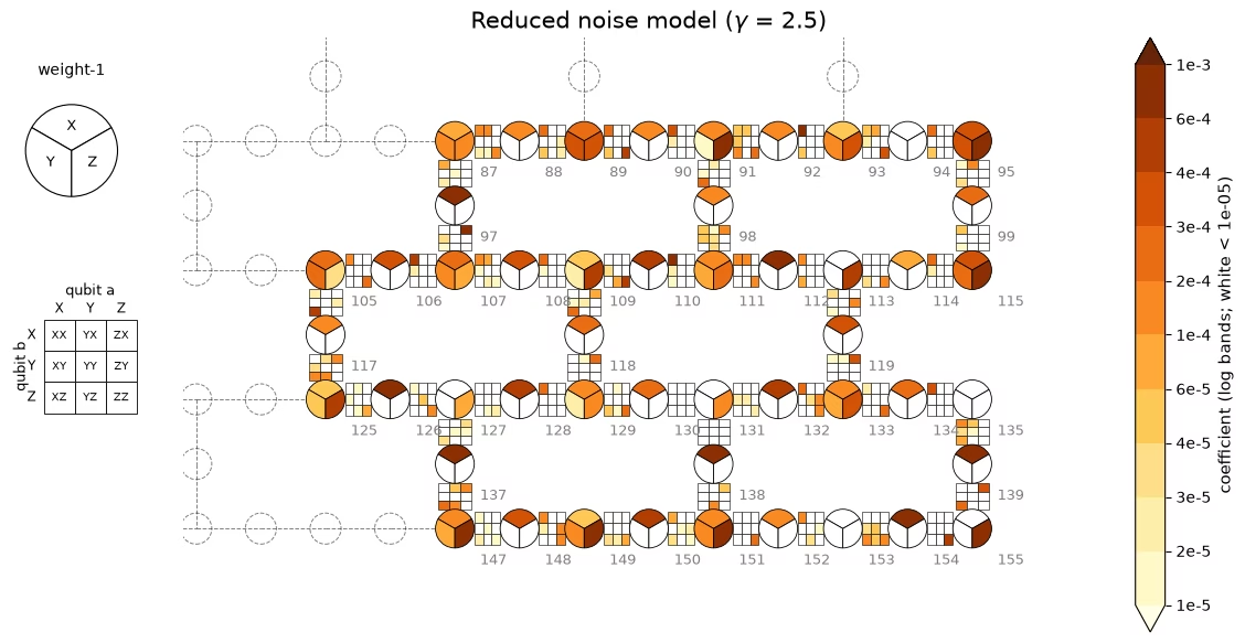
Každá kontrola symetrie je schopna detekovat určitou podmnožinu generátorů chyb v modelu šumu, což znamená, že tyto chyby nemusíš potlačovat. Zde vytvoříme masku nad detekovatelnými generátory šumu pomocí funkce create_postselected_noise_mask z qiskit_mitigation. Tato maska bude použita k ořezání modelu šumu o detekovatelné členy před provedením PEC. Provedení PEC vzhledem k ořezanému modelu šumu může poskytnout konvergované střední hodnoty za zlomek nákladů na vzorkování potřebných k provedení PEC na plném modelu šumu, jak je znázorněno na mapách modelu šumu výše.

Mapa níže je nakreslena na stejné barevné škále jako naučený model výše, přičemž zachovává pouze generátory chyb, které kontroly nedokážou detekovat. Vidíme, že z modelu byl odstraněn velký počet generátorů chyb a režie vzorkování výrazně klesla. Režie vzorkování pro spuštění PEC na ořezaném modelu šumu je $\gamma^2=2.5^2\approx6.3$, což je zhruba 16násobné snížení oproti režii potřebné k potlačení plného šumového kanálu.

from qiskit.quantum_info import Pauli
from qiskit_mitigation.noise import create_postselected_noise_mask

SHOTS_PER_RAND = 64  # shots per PEC randomization
N_RAND = 23_054  # PEC randomizations per experiment
MAX_PAIR_RATE = 0.02  # Max value of any coupler's summed two-qubit error rate

# The detectors are virtual Pauli-Z's representing the measurements on the mediator qubits
# We can find the set of detectable noise generators in the model for each detector by conjugating
# it backward through the circuit and calculating what generators it anti-commutes with.
detectors = [
    Pauli("I" * (boxed.num_qubits - 1 - q) + "Z" + "I" * q)
    for q in layout[n_data:]
]
# Detectable generators are handled by postselection; prune them from the model for PEC
local_scales, gamma2_post = create_postselected_noise_mask(
    boxed, noise_maps, detectors
)
gamma_post = gamma2_post**0.5
print(f"gamma PEC {gamma:.2f} | gamma QED+PEC {gamma_post:.2f}")

# Kill the job if any coupler's summed rate exceeds MAX_PAIR_RATE
pair_lam = {}
for m in noise_maps.values():
    for _, qs, r in m.to_sparse_list():
        if len(qs) == 2:
            pair_lam[tuple(sorted(qs))] = (
                pair_lam.get(tuple(sorted(qs)), 0.0) + r
            )
assert (
    max(pair_lam.values()) < MAX_PAIR_RATE
), f"kill: degraded coupler {max(pair_lam, key=pair_lam.get)}"

# Detectability depends on circuit position, so record each site's 0/1 scales by layer
site_ref = {
    a.modifier_ref: a.ref
    for inst in boxed.data
    if inst.operation.name == "box"
    and (a := get_annotation(inst.operation, InjectNoise))
    and a.ref
}
sites = sorted(local_scales, key=lambda s: int(s[1:]))
mit["site_scales"] = np.stack([local_scales[s] for s in sites])
mit["site_layer"] = np.array(
    [list(noise_maps).index(site_ref[s]) for s in sites]
)
mit["gammas"] = np.array([gamma, gamma_post])
draw_noise_map(mit, backend, reduced=True)

gamma PEC 10.08 | gamma QED+PEC 2.52

Vzorkujte obvod detekující chyby

Zde vzorkujeme 49qubitový Isingův obvod detekující chyby. Povolíme Pauliho twirling a nemarkovské kontroly chyb, ale neprovádíme vzorkování PEC. Tyto vzorky použijeme k výpočtu základních středních hodnot i středních hodnot pouze s detekcí chyb.

# Baseline = the ED+PEC template itself at noise scale 0, i.e. twirling only
program_tw = QuantumProgram(shots=100)
program_tw.append_samplex_item(
    template_checked,
    samplex=samplex,
    shape=(1000, 1),
    samplex_arguments={
        "pauli_lindblad_maps": dict(noise_maps),
        basis_key: meas_basis,
        **{f"noise_scales.{k}": 0.0 for k in local_scales},
    },
)
job_tw = Executor(session, options=executor_options).run(program_tw)

Vzorkujte obvod detekující chyby s PEC

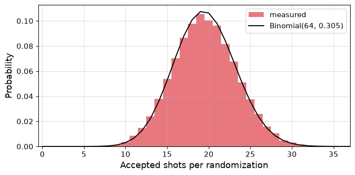
Nyní vzorkujeme znovu a zahrneme randomizace PEC k potlačení šumu, který kontroly symetrie nedokáží detekovat. Tyto vzorky budou použity k výpočtu středních hodnot pomocí kombinace detekce chyb s PEC. Níže vykreslíme přijaté shoty na randomizaci PEC oproti binomickému rozdělení při průměrné míře přijetí. Vidíme, že přijetí nekoreluje s vzorkovanou instancí obvodu, protože QED+PEC injektuje pouze nedetekovatelné Pauliho operátory, které komutují s měřeními každého mediátorového qubitu.

def launch(session, template, samplex, samplex_args, n_rand, shots_per_rand):
    """Sample `n_rand` randomizations of `template` on `session` in <=100k-randomization jobs; returns the jobs."""
    jobs = []
    for start in range(0, n_rand, 100_000):
        program = QuantumProgram(shots=shots_per_rand)
        program.append_samplex_item(
            template,
            samplex=samplex,
            samplex_arguments=samplex_args,
            shape=(min(100_000, n_rand - start), 1),
        )
        jobs.append(Executor(session, options=executor_options).run(program))
    return jobs

# Reduced PEC
args_post = {
    "pauli_lindblad_maps": dict(noise_maps),
    basis_key: meas_basis,
    **{f"noise_scales.{k}": -1.0 for k in local_scales},
    **{f"local_scales.{k}": v for k, v in local_scales.items()},
}
# PEC on the full noise model
args_van = {
    "pauli_lindblad_maps": dict(noise_maps),
    basis_key: meas_basis,
    **{f"noise_scales.{k}": -1.0 for k in local_scales},
}

# Run sampling jobs
jobs = launch(
    session, template_checked, samplex, args_post, N_RAND, SHOTS_PER_RAND
)
jobs_van = launch(
    session, template_checked, samplex, args_van, N_RAND, SHOTS_PER_RAND
)
outs = [j.result()[0] for j in jobs]
outs_van = [j.result()[0] for j in jobs_van]
(out_tw,) = job_tw.result()
session.close()

Shromážděte vzorky a ověřte, že randomizace PEC komutují s měřeními na mediátorových qubitech a neovlivňují statistiku postselekce.

def bitflip_mask(out, selector):
    """Per-shot True/False for job result `out`: shot passes `selector`'s non-Markovian error checks."""
    regs = {
        k: np.asarray(out[k])
        for k in out
        if not k.startswith(("measurement_flips", "pauli_signs"))
    }
    return selector.compute_mask(regs, "edge", mode="post")

def symmetry_mask(out):
    """Per-shot True/False for job result `out`: every twirl-corrected symmetry check reads 0."""
    return ~(
        np.asarray(out["check"]) ^ np.asarray(out["measurement_flips.check"])
    ).any(axis=-1)

def keep_mask(out, selector):
    """Per-shot True/False for job result `out`: shot passes both check types."""
    return symmetry_mask(out) & bitflip_mask(out, selector)

def fracs(out_list, selector):
    """Fractions of shots across the job results in `out_list` passing [no, non-Markovian error, symmetry, both] checks."""
    bf = np.concatenate([bitflip_mask(o, selector) for o in out_list])
    sy = np.concatenate([symmetry_mask(o) for o in out_list])
    return [1.0, bf.mean(), sy.mean(), (bf & sy).mean()]

mask_post = np.concatenate([keep_mask(o, selector) for o in outs])

# Collect the sampled data alongside the learned model, in the form the figure helpers expect
mit.update(
    ps_fracs=np.array(
        [
            fracs([out_tw], selector),
            fracs(outs_van, selector),
            fracs(outs, selector),
        ]
    ),
    acc_counts_post=np.squeeze(mask_post).sum(axis=-1),
    data_tw=np.asarray(out_tw["data"]),
    flips_tw=np.asarray(out_tw["measurement_flips.data"]),
    mask_tw=keep_mask(out_tw, selector),
    data_post=np.packbits(
        np.concatenate([np.asarray(o["data"]) for o in outs]), axis=-1
    ),
    flips_post=np.concatenate(
        [np.asarray(o["measurement_flips.data"]) for o in outs]
    ),
    signs_post=np.concatenate([np.asarray(o["pauli_signs"]) for o in outs]),
    mask_post=mask_post,
    data_van=np.packbits(
        np.concatenate([np.asarray(o["data"]) for o in outs_van]), axis=-1
    ),
    flips_van=np.concatenate(
        [np.asarray(o["measurement_flips.data"]) for o in outs_van]
    ),
    signs_van=np.concatenate(
        [np.asarray(o["pauli_signs"]) for o in outs_van]
    ),
    mask_van=np.concatenate([bitflip_mask(o, selector) for o in outs_van]),
)

# Plot the PEC bias check
plot_postselection(mit)

Vypočítejte střední hodnoty a porovnejte strategie

Nakonec vypočítáme všechny střední hodnoty pomocí pomocné funkce executor_expectation_values z qiskit-mitigation, která za nás aplikuje překlopení měření, masky postselekce, faktory přeškálování TREX a znaménka kvazipravděpodobnosti.

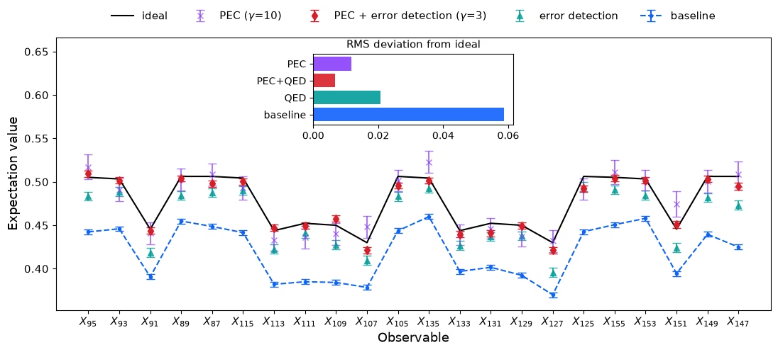
Horní graf: Vidíme, že obě varianty PEC konvergují, ale QED+PEC dosáhne pásma $\pm 0.025$ s méně randomizacemi a užšími chybovými úsečkami. Reziduální zkreslení ve výpočtu QED+PEC je pod 0.01 a lze ho přičíst kombinaci neshody modelu šumu, driftu qubitů v čase a efektů z nemodelovaných zdrojů šumu.

Dolní graf: Průběžný odhad zprůměrované $\langle X \rangle$ přes místa, jak se randomizace akumulují, při použití shodného počtu shotů na randomizaci pro obě varianty PEC. PEC + detekce chyb se ustálí v pásmu během několika tisíc randomizací; samotné PEC, které platí plnou režii vzorkování, vyžaduje mnohem více randomizací ke konvergenci.

from qiskit.quantum_info import SparsePauliOp
from qiskit_mitigation.utils import executor_expectation_values

gamma, gamma_post = mit["gammas"]
basis_map = {Pauli("X" * n_data): [SparsePauliOp(o) for o in observables]}
rescale = dict(zip(observables, mit["trex_rescale"], strict=True))

def evs(bits, basis_map, **kwargs):
    """Per-site (means, standard errors) from boolean shot data `bits` of shape (rands, 1, shots, n_data)."""
    out = executor_expectation_values(
        bits, basis_map, None, avg_axis=(0, 1), **kwargs
    )
    return np.array([m for m, _ in out]).ravel(), np.sqrt(
        [v for _, v in out]
    ).ravel()

def unpack(mit, prefix, n_data):
    """Restore `mit[f"data_\{prefix\}"]` from packed bytes to booleans of shape (rands, 1, shots, n_data)."""
    return np.unpackbits(mit[f"data_{prefix}"], axis=-1)[..., :n_data].astype(
        bool
    )

unmit_tw, unmit_tw_err = evs(
    mit["data_tw"], basis_map, measurement_flips=mit["flips_tw"]
)
ed_tw, ed_tw_err = evs(
    mit["data_tw"],
    basis_map,
    measurement_flips=mit["flips_tw"],
    postselect_mask=mit["mask_tw"],
    rescale_factors=rescale,
)
post, post_err = evs(
    unpack(mit, "post", n_data),
    basis_map,
    measurement_flips=mit["flips_post"],
    pauli_signs=mit["signs_post"],
    postselect_mask=mit["mask_post"],
    rescale_factors=rescale,
)
pec, pec_err = evs(
    unpack(mit, "van", n_data),
    basis_map,
    measurement_flips=mit["flips_van"],
    pauli_signs=mit["signs_van"],
    postselect_mask=mit["mask_van"],
    rescale_factors=rescale,
)

# effective ED+PEC overhead measured from the data: accepted shots per signed accepted shot
signs_post = 1 - 2 * (np.squeeze(mit["signs_post"]).sum(axis=-1) % 2)
gamma_eff = (
    mit["mask_post"].sum()
    / (signs_post * np.squeeze(mit["mask_post"]).sum(axis=-1)).sum()
)

print(
    f"gamma PEC {gamma:.2f} | gamma QED+PEC {gamma_post:.2f} (model) / {gamma_eff:.2f} (data) | "
    f"QED survival {mit['mask_tw'].mean():.3f} | QED+PEC survival {mit['mask_post'].mean():.3f} | "
    f"mean QED+PEC err {post_err.mean():.4f}"
)
plot_final(
    obs_exact,
    (unmit_tw, unmit_tw_err),
    (ed_tw, ed_tw_err),
    (pec, pec_err),
    (post, post_err),
    (gamma, gamma_post),
    x_labels(layout, n_data),
    "",
)

gamma PEC 10.08 | gamma QED+PEC 2.52 (model) / 2.51 (data) | QED survival 0.304 | QED+PEC survival 0.305 | mean QED+PEC err 0.0037

plot_convergence(mit, obs_exact, n_data)